New PCA-based Compression Method for Natural Color Images New PCA-based Compression Method for Natural Color Images

New PCA-based Compression Method for Natural Color Images

A. Abadpour

S. Kasaei

Mathematics Science School, Sharif University of Technology

Computer Engineering School, Sharif University of Technology

Abstract

The color information in a natural image can be considered as a highly correlated vector space. This high correlation is the first motivation towards using linear dimensionality reduction methods like principal component analysis for the sake of data compression. In this paper new color image decomposition methods are proposed and compared experimentally. Using a newly proposed gray-scale image colorizing method, a new compression method is proposed for natural color images, that while reducing the spectral redundancy of natural color images, it leaves the spatial redundancy unchanged, to be handled with a specialized spatial-compression method independently, and is proved to be highly efficient.

Principle Component Analysis Color Image ProcessingQuad-tree DecompositionColor Image Compression.

1 Introduction

Color is the way the human visual system (HVS) perceives a part of the electromagnetic spectrum approximately between 380nm and 780nm. A color space is a method to code a wave in this range.

Although, due to practical reasons, the Red-Green-Blue (RGB) color space is widely used, when dealing with natural images it suffers from the high correlation between its components [1]. Furthermore, the RGB color space has proved to be psychologically not intuitive [2] and perceptually non-uniform [2,3]. Different color spaces are proposed in the literature [4] but there are only a few color space comparison articles available. A recent work [5] considers the effects of color space selection on the skin detection performance, reporting that non of the eight color spaces of normalized RGB (NRGB), CIE-XYZ, CIE-La^*b^*, HSI, spherical coordinate transform (SCT), YC_bC_r, YIQ, and YUV respond better. Another paper [6] investigates five color spaces including RGB, YIQ, CIE-L^*A^*B^*, HSV, and Opponent color and experimentally compares them in terms of human ability to produce a given color by changing the coordinates in a given color space. A new paper [7] compares the eleven color spaces of YC_bC_r, NTSC, PAL, HDTV, UVW, CIE-XYZ, DCT, DHT, K₁K₂K₃ and KLT and the original reversible color transform (ORCT) in terms of image coding. In this paper "the primary objective is to find a linear color transform that maps integers to integers and reversible, yield good objective image quality in the case of lossy compression". In [8], the authors compared the twelve standard color spaces of RGB, CMYK, HSI, I₁I₂I₃, CIE-La^*b^*, CIE-L^*H^oC^*, CIE-Lu^*v^*, CIE-XYZ, YC_bC_r, YIQ, and YUV, according to results of spotting colors, in a simple image containing eight different objects with different colors. Also, taking advantages of principle component analysis, a new adaptive color space called PCA-PLAC is proposed which performs the job more accurate and more stable compared to the standard color spaces under investigation [8].

Although many modern imaging systems are still producing gray-scale images, color-images are more preferred due to the larger amount of information contained by them. Computing the gray-scale representation of a color image is a trivial task, but when dealing with the inverse problem, the task shows itself as a more complicated job; that should be performed with some levels of human intervention. Authors have performed a widespread search in the literature containing personal contact to the authors of the very few papers found in the field. Rather than the classic pseudocoloring task proposed by Gonzalez [9], The only noteworthy works are published by Welsh [10], Yan [11], and a newly proposed PCA-based gray-scale image colorizing method [8]. The methods are compared both subjectively and quantitatively [8] and the new method is proved to be dominant.

Quad-tree decomposition is a method for splitting an image into homogenous sub-blocks [12]. Defining the whole image as a single block, the method is performed according to some problem-specific homogeneity criteria. Each block is examined to check wether it is homogenous or not. If it is not, then it will be split into four same-sized blocks. The method terminates when there is no other blocks to be split or when all blocks to be split are smaller than a pre-selected size. The minimum size of the blocks is set, to avoid over segmentation. Work on generalization of quad-tree decomposition has been performed, both on dimension [13] and shape [14] of the blocks. Using rectangular blocks is known to have many benefits. Firstly, performing block-wise operations in rectangular regions is computationally inexpensive. In addition, more complicated blocks, as triangles, perform division operator on spatial variables which leads to more round-off and misalignment errors. When using the simple one-split-to-four rule, the number of blocks desperately increases by factor of four. Having in mind that increasing number of blocks declines the performance of post-processes like recomposition and compression, the need for a better splitting method arises.

The idea of reducing the color space dimension is not a new idea; many researchers have reported benefits of illumination coordinate rejection [5,1]. The principle component analysis (PCA) [15,16,17] is widely used in signal processing, statistics, and neural networks. In some areas, it is called the (discrete) Karhunen-Leove transform (in continuous case) or the Hotelling transform (in discrete case). The basic idea behind the the PCA is to find the components {s₁ ¼s_n}, so that they determine the maximum amount of variance possible by n linearly transformed components (s_i=w_i^Tx). In practice, the computation of w_i can be simply accomplished using covariance matrix C = E{ (x-[`x]) (x- [`x])^T }. , where w_n is the eigenvector of C corresponding to the n^th largest eigenvalue [15]. The basic goal in PCA is to reduce the data dimension. Thus, one usually chooses n << m. Indeed, it can be proven that the representation given by PCA is an optimal linear dimension reduction technique in the mean-square sense. Such a reduction in dimension has important benefits. First, the computational cost of the subsequent processing stage is reduced. Second, noise can be reduced; as the data not contained in the n first components may be mostly due to noise [15]. Using PCA for color image processing is not a new idea. A recent work [18] proposes a new approximation for PCA and a new set of methods for performing color image processing primitives of edge-detection, sharpening and compression. Although due to the computation cost of principle components, an accurate fast approximation seems useful, but according to the probabilistic characteristic of data, precautions must be made to avoid noise sensitivity of the approximation. The paper [18] proposes to use the "color vector of the central pixel of the window before constructing the corresponding covariance matrix" for the purpose of "computation efficiency" in contrast with our proposal of using the average of the window. Using such deterministic noise-dependant values in the spatial map must be avoided. Also in the proposed approximation, the direction of the first principle component is selected as the vector starting at mean, ending at the furthest point of the data cloud. Having in mind the scattered pattern of the color vectors in a natural image, even containing some completely irrelevant points, it is clear that the proposed method [18] is noise-dependent to great extends.

In this paper the three notations éxù, ëxû, and /x/ are used as the smallest integer larger than x, the largest integer smaller than x, and the nearest integer to x, respectively.

2 Proposed Methods

2.1 Quad-tree Decomposition of Color Images

We propose thresholds [e\tilde]_R [8] as a region homogeneity criteria:

h(R)=

ì
ï
í
ï
î

1,|

| £ e₁

0, otherwise

(1)

where e₁ is a user-selected parameter, mostly in the range [1... 10]. The minimum size of blocks for a W×H image is set to d_x×d_y, where:

d_x=éW×2^-(r-1)ù

(2)

d_y=éH×2^-(r-1)ù

(3)

Tree depth (r) is either asked from the user or computed as:

r = ëlog₂

min

{W,H}û

(4)

During the decomposition stage, all the information is saved as a 13×N matrix called L, where N is the number of the blocks and each row of L consists of x₁, y₁, x₂, y₂, h₁, h₂, h₃, v₁, v₂, v₃, [e\tilde]_R, and two reserved parameters.

The number of blocks must be considered thoughtfully. If we define N_n as the number of blocks after n passes of splitting, it is clear that for fully scattered images, while setting e₁=0 the algorithm will give N_n=4^n-1.

According to the inflated number of blocks produces in ordinary quad-tree decomposition method, two new bi-tree decomposition methods are proposed. Rather than the one-to-four rule in quad-tree decomposition, here any non-homogenous block is split into two blocks. Assuming that the block R is not enough homogenous, In the first method called bi₁₁-tree decomposition, two sets of alternatives for decomposition are proposed (see Figure 1). If [e\tilde]_R₁+[e\tilde]_{\acute R₁} < [e\tilde]_R₂+[e\tilde]_\acuteR₂ the block is split vertically and it is split horizontally otherwise. In the second proposed method, called bi₁₂-tree decomposition, four sets of alternatives are investigated (see Figure 2). The method corresponding to the minimum of { [e\tilde]_R₁+[e\tilde]_{\acute R₁}, [e\tilde]_R₂+[e\tilde]_{\acute R₂}, [e\tilde]_R₃+[e\tilde]_\acuteR₃, [e\tilde]_R₄+[e\tilde]_{\acute R₄}} is the winner. In the two new proposed methods, the rectangular clipping is reserved while the block shape changes to best fit the image. Experimental results are discussed in Section 3.1.

0.5cm
Picture Omitted
Figure 1: Proposed bi₁₁-tree.

0.5cm
Picture Omitted
Figure 2: Proposed bi₁₂-tree.

2.2 Color Image Compression

Based on the proposed image decomposition method (See Section 2.1), a new compression method for color images of natural scenes is proposed; As a sub-sampling stage presents in the process, the image is firstly filtered using an ideal low-pass filter to avoid further aliasing:

H₁(z₁,z₂)=

ì
ï
í
ï
î

1,|z₁| <

2d_x

,|z₂| <

2d_y

0,otherwise

(5)

where d_x and d_y are defined in (2). Let's call the filtered version of the original image I, as [I\tilde].

One of the decomposition methods proposed in Section 2.1 are performed on [I\tilde], resulting in the 13×N matrix L. It is clear that L can be compressed, to be stored in 12N bytes, each row contains {x₁,y₁, /log₂[W/(x₂)]/, /log₂[Y/(y₂)]/}È{h₁, h₂, h₃, v₁, v₂, v₃}, which are all stored as 0... 255 variables, rather than x₁, y₁ that are stored as 0... 65535 variables. Assuming that we are working on a W×H color image, the size of the file is 3WH bytes. We propose computing the gray-scale version of the image (contains WH bytes of data), and replacing the least significant bit (LSB) of all bytes with the information in L. It is clear that, the user does not perceive the diversified bit. The image now contains ⁷/₈WH+11N bytes of data. If the image is not too scattered the compression ratio will be about 3. To say more precisely, the compression ratio is less than [24/7] @ 3.428, depending on the image complexity.

Now we propose the reconstruction method to compute the uncompressed version of data in color representation. A very simple reconstruction method is using [(h)\vec] and [v\vec] values of any block to colorize its contents [8]. Here we propose a better method that has shown better quantitative and subjective results. We call the simple method as the zero method while the next method is called the plus method.

Assuming the two 3×W ×H matrices E and V, and the W ×H matrix C, we set all elements in E, V, and C to zero. Scanning L, that we have extracted from the compressed data row by row, we fill the matrices in this way: When processing the block (x₁,y₁)-(x₂,y₂) with the two describing vectors [(h)\vec]=[

h₁

h₂

h₃

]^T and [v\vec]=[

v₁

v₂

v₃

]^T, for any x Î [x₁... x₂] and y Î [y₁... y₂] that d_x|x and d_y|y and for all i Î {1,2,3}, we set E[i,w_{d_x}(x),w_{d_y}(y)] = h_i and V[i,w_{d_x}(x),w_{d_y}(y)]=v_i. Also we set C[w_{d_x}(x),w_{d_y}(y)]=1. Where w_{d_x}(x) defined as:

w_a(x)=a×/

(6)

is used to align the points in a d_x×d_y grid. Due to occurrence of round-off, some samples of E and V align the d_x×d_y grid are lost. C is used to compensate this information-loss. When setting an element of E, say E(i,x,y), the set defined as:

{(u,v)||u-x| £ d_x, |v-y| £ d_y }

(7)

is searched for zero values of C align the d_x×d_y grid. If such points are found, the values of E(i,x,y) and V(i,x,y) are copied into appropriate cells of E and V respectively. Now E and V, contain samples of the signals [E\tilde] and [V\tilde] sampled by a cartesian grid (d_x×d_y). Reconstruction of [E\tilde] and [V\tilde] is easily performed using the ideal low-pass filter defined as:

H₂(z₁,z₂)=

ì
ï
í
ï
î

d_xd_y,|z₁| <

2d_x

,|z₂| <

2d_y

0,otherwise

(8)

Using G (the contents of the 7 most significant bits (MSB) of the compressed image) as the source image and [E\tilde], [V\tilde] as the color content, by applying either of the two colorizing methods proposed in [8], the color information is reproduced simply. It is clear that the proposed compression method is independent of the method that has produced L, either be quad-tree decomposition or bi-tree decomposition. Experimental results are shown in Section 3.2.

3 Performance Evaluation

All algorithms are developed in MATLAB 6.5, on an 1100 MHz Pentium III personal computer with 256MB of RAM. The code for all algorithms is available online at http://math. sharif. edu/ ~ abadpour/code.html.

3.1 Quad-tree Decomposition of Color Images

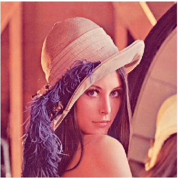
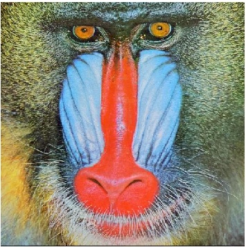
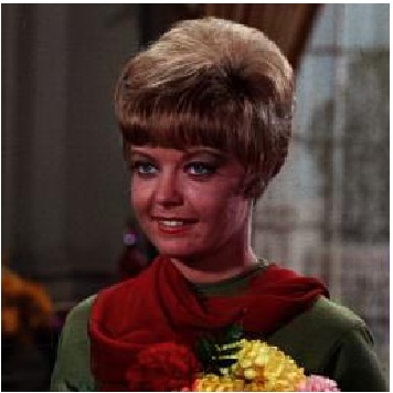
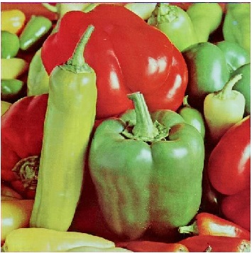
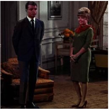
To compare the results of the three proposed decomposition methods, six standard images of Peppers, Couple, Girl, Lena, Airplane, and Mandrill are decomposed by setting e₁=1¼10 for each method (30 decompositions per image). In all tests when the value of r is not restricted, it is computed as described in (4). Figure 3 shows results of the proposed decomposition methods on three standard images of Lena, Airplane, and Peppers (As three ordinary, simple, and complex samples respectively). The values of e₁, t, N, and r are denoted in the caption of Figure 3 for each sample along with the method used to decompose the image. 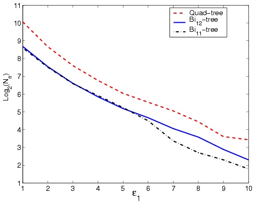In order to compare number of blocks made in the three proposed methods in each iteration of the algorithm, the standard image Lena is decomposed by setting e₁=2. Results are shown in Figure 4. Also the same image is decomposed with different values of e₁ in the range of [1¼10]. 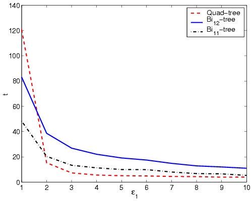The results are shown in Figure 5-a. Required time to decompose the standard image Mandrill with different values of e₁ in the range of [1¼10] are shown in Figure 5-b.


(a)	(b)	(c)

(d)	(e)	(f)

(g)	(h)	(i)

(j)	(k)	(l)

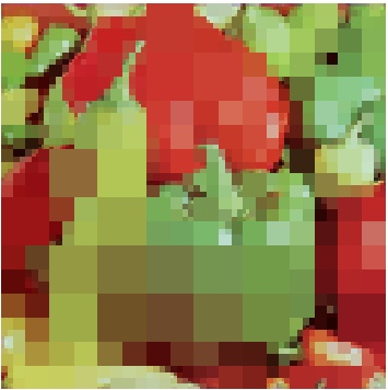
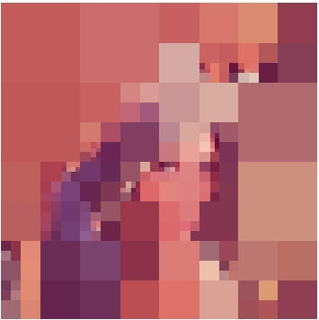
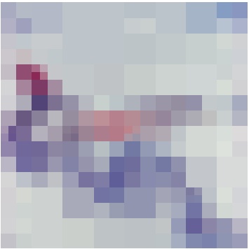
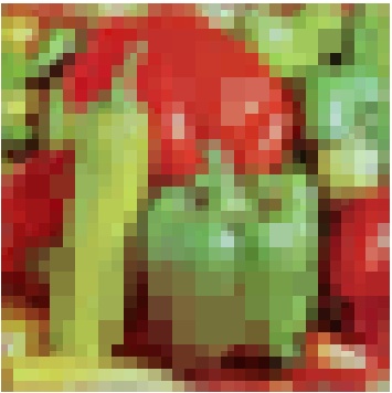
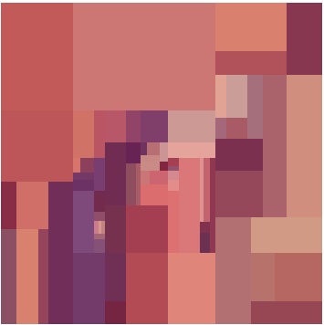
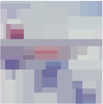
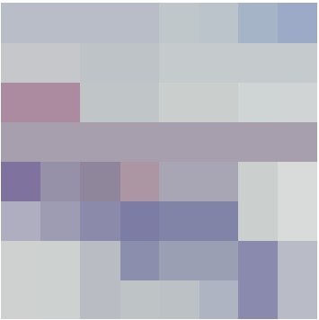
Figure 3: Results of the proposed decomposition methods on Lena, Airplane, and Peppers. (a)-(f): quad-tree decomposition, (g)-(i):bi₁₂-tree decomposition, and (j)-(l): bi₁₁-tree decompositionParameters: [e₁, t, N, r], (a) [3, 5s, 295, 6] (b) [2, 5s, 214, 6] (c) [5, 7s, 1462, 8] (d) [5, 5s, 205, 7] (e) [1, 5s, 193, 5] (f) [2, 7s, 1054, 6] (g) [5, 18s, 77, 7] (h) [1, 20s, 86, 5](i) [2, 24s, 324, 6] (j) [5, 10s, 79, 7] (k) [1, 10s, 36, 5] (l) [2, 1s, 172, 6]

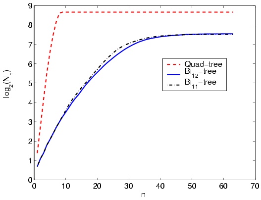
Figure 4: Block count growth in three proposed decomposition methods performed on standard image Lena.


(a)	(b)

Figure 5: Results of the proposed decomposition methods for different values of e₁ performed on standard image Lena. (a) Block count, (b) elapsed time

Comparing the curves in Figure 4 shows that the proposed quad-tree decomposition method converges in much lower number of iterations compared with the proposed bi₁₁-tree and bi₁₂-tree decomposition methods, Whilst bi₁₂-tree has the most convergence time. In addition comparing the final values shows that final number of blocks in the two bi-tree methods are almost the same, while with the same e₁, quad-tree has produced twice number of blocks. Considering the number of blocks (Which rules the performance of the method processing the blocks, like recomposition or compression), it is clear that bi-tree methods are better than the quad-tree method. Figure 5-a shows that the number of blocks when treated in logarithmic scale, relates almost linearly to the value of e₁. The decline in the number of blocks in higher values of e₁ for quad-tree and bi₁₁-tree are also thoughtful. While for compression purposes, one selects lower values of e₁, higher values are appropriate for compression usages. Figure 5-a shows that bi₁₁-tree is a better choice for segmentation compared to quad-tree and bi₁₂-tree methods.

As expected, quad-tree decomposition is averagely faster than the bi-tree methods (see Figure 5-b). This is not strange when considering the excessive computation of alternative blocks in bi-tree methods. While bi₁₁-tree performs four homogeneity computations, bi₁₂-tree performs eight ones, describing the lower speed of bi₁₂-tree compared to bi₁₁-tree. The sudden increase of elapsed time in quad-tree decomposition for values of e₁ < 2 happens in all samples. As low values of e₁ are better responding to compression, it is clear the bi₁₁ is an appropriate choice for compression.

The above discussion leads to two promising results. Firstly bi₁₁-tree decomposition over-performs the two other methods in compression and recomposition usages, both in terms of elapsed time and number of blocks. Secondly, it is clear that the more complicated bi₁₂-tree decomposition not only is not responding better than bi₁₁ but also has less performance. the motivation towards bi₁₂-tree decomposition is to define a new structure that inherits the brilliant one-to-two splitting characteristic of bi₁₁-trees along with more adaptivity. The results show that with less time efficiency, bi₁₂-tree is not responding meaningfully better than bi₁₁-tree. This desperate result avoids us to define new definitions of bi-tree decomposition with more complicated alternatives.

3.2 Color Image Compression

To compare the results of the proposed compression method, 6 standard images of Peppers, Couple, Girl, Lena, Airplane, and Mandrill are compressed by setting e₁=1¼10 for each of the three proposed decomposition methods (30 compressions per image). In all tests r is computed as described in (4). Figure 6 shows nominal results of the standard images. The PSNR and l values are denoted in the caption. 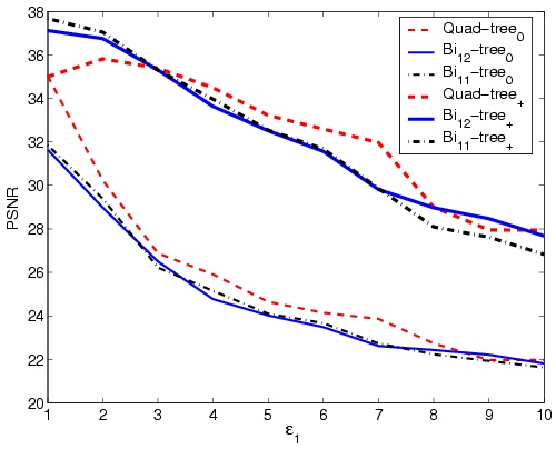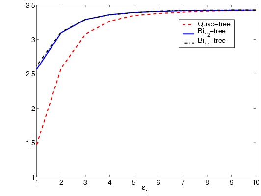For different values of e₁ Î [0¼10], Figure 7-a shows values of the PSNR₀ and the PSNR₊ for the standard image Lena and Figure 7-b shows the respective compression ratio results.


(a)	(b)	(c)

(d)	(e)	(f)

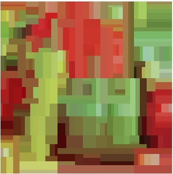
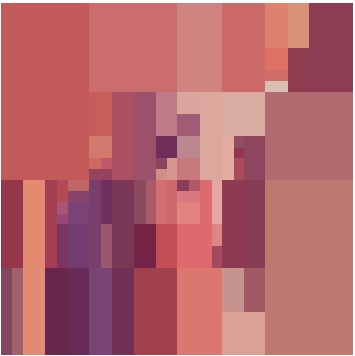
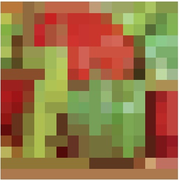
Figure 6: Results of the proposed compression method. (a) Lena: PSNR=35, l = 3.13 (b) Mandrill:PSNR=31, l = 1.79 (c) Girl: PSNR=35, l = 2.86 (d) Airplane:PSNR=35, l = 3.13 (e) Peppers:PSNR=31, l = 2.50 (f) Couple:PSNR=36, l = 3.13


(a)	(b)

Figure 7: Results of the proposed compression method on standard image Lena for different values of e₁. (a)PSNR₀ and PSNR₊, (b) Compression ratio

The sample images of Figure 6 are subjectively desiring. Authors have performed a very simple but efficient test. Among the 31 people participating in a subjective test, no one was able to distinguish between the compressed images and the original ones. Even the authors were many times in doubt, wether they are watching the original image or the compressed one.

l values must be considered precisely. As the proposed compression method works on spectral redundancy, the marginal value of l is 3. Having in mind that almost no spatial redundancy decreasing have performed in this method, it is clear that any gray-scale image compression method can be serialized with our proposed method, to compress the 7-bit, G matrix. The point is the definitely independence of the spatial and spectral compression methods.

As it is clear in Figure 7-a, bi₁₁-tree over-performs the bi₁₂-tree in terms of PSNR. This result complies with the discussions in Section 3.1. Although quad-tree has given better PSNR values compared with bi-tree methods for higher values of e₁, considering that the high compression ratios are gained in lower values of e₁, where bi₁₁-tree is the dominant method, proves that bi₁₁-tree is the best selection for compression. A noticeable fact in Figure 7-a is the same value of the PSNR for quad-tree in e₁=1. As with decreasing values of e₁, quad-tree decomposition process converges to the ordinary uniform sampling, the proposed compression method reduces to a simple sub-sampling of color information. the more than 2 steps difference between values of the PSNR of quad-tree and bi₁₁-tree at e₁=1 shows the over-performance of the proposed bi₁₁-tree decomposition. The higher than 3 values of compression ratio with the PSNR value of more than 35 qualifies the performance of our proposed compression method.

4 Conclusion

Quad-tree decomposition of gray-scale images is not a new method, but in this paper a new method for decomposition of color images is proposed based on a previously proposed region homogeneity criteria [8]. Although a few other decomposition methods are proposed in the literature [14], by they lack the simplicity of quad-trees. Here, two new bi-tree decomposition methods are proposed that reduce the number of blocks considerably while using rectangular blocks, resulting in algorithm simplicity.

A new color image compression method is proposed that leaves the spatial redundancy almost unchanged while reducing the spectral redundancy almost entirely. The method which is based on the proposed decomposition methods, compresses color images with the factor of three while giving high values of PSNR. Having in mind that the theoretical value for an spectral-based compression method is three, the brilliancy of our proposed compression method is clear.

Acknowledgement

The first author wishes to thank Mrs. Azadeh Yadollahi for her encouragement and invaluable ideas.

References

[1]: P. H., Representation of color images in different color spaces, in: S. Sangwine, R. Horne (Eds.), The color image processing handbook, Chapman and hall, London, 1998, pp. 67-90.
[2]: CIE, CIE. International Lighting Vocabulary, CIE Publications, 4th edition, 1989.
[3]: I. Tastl, G. Raidl, Transforming an analytically defined color space to match psychophysically gained color distances, in: the SPIE's 10th Int. Symposium on Electronic Imaging: Science and Technology, Vol. 3300, San Jose, CA, January 1998, pp. 98-106.
[4]: K. N. Plataniotis, A. N. Venetsanopoulos, Color Image Processing and Applications, Springer-Verlag, Heidelberg-New York, 2000.
[5]: L. V. T. Min C. Shin, Kyong I. Chang, Does color space transformation make any difference on skin detection?, http://citeseer.nj.nec.com/542214.html.
[6]: W. B. C. Micheal W. Schwarz, J. C. Beaty, An experimental comparison of rgb, yiq, lab, hsv and opponent color models, ACM Transaction on Graphics 6 No. 2 (April 1987) 123-158.
[7]: P. Hao, Q. Shi, Comparative study of colortransforms for image coding and derivation of integer reversible color transform, 2000, pp. 224-227.
[8]: A. Abadpour, S. Kasaei, New principle component analysis based methods for color image processing, Submitted to Visual Communication and Image Representation Journal.
[9]: G. R.C., W. P., Digital Image Processing, Addison-Wesley Publications, Reading, MA., 1987.
[10]: M. A. Tomihisa Welsh, K. Mueller, Transferring color to grayscale images, in: ACM SIGGRAPH 2002, San Antonio, July 2002, pp. 277-280.
[11]: M. S. K. Wei-Qi Yan, Colorizing infrared home videos, ICME 2003 1 (2003) 97-100.
[12]: H. Samet, Region representation: Quadtrees from boundary codes, Comm. ACM 21 (March 1980) 163:170.
[13]: H. J. Christos Faloutsos, Y. Manolopoulos, Analysis of the n-dimensional quadtree decomposition for arbitrary hyperrectangles, IEEE Transaction on Knowledge and Data Engineering 9, No. 3 (May/June 1997) 373-383.
[14]: M. Yazdi, A. Zaccarin, Interframe coding using deformable triangles of variable size, 1997, pp. 456-459.
[15]: A. Hyvarinen, Independent component analysis: Algorithms and applications, IEEE transaction on Neural Networks.
[16]: I. T. Jolliffe, Principal Component Anslysis, Springer-Verlag, Heidelberg-New York, 1986.
[17]: M. Kendall, Multivariate Analysis, Charlas Griffin and Co., 1975.
[18]: S.-C. Cheng, S.-C. Hsia, Fast algorithm,s for color image processing by principal component analysis, Jurnal of Visual Communication and Image Representation 14 (2003) 184-203.

File translated from T_EX by T_TH, version 3.72.
On 01 Aug 2006, 13:34.