Video--on--Demand Network Design And Maintenance Using Fuzzy Optimization

Video-on-Demand Network Design And Maintenance Using Fuzzy Optimization

Arash Abadpour, Attahiru Sule Alfa, and Jeff Diamond ¹

Abstract

Video-on-Demand (VoD) is the entertainment source which, in the future, will likely overtake regular television in many aspects. Even though many companies have deployed working VoD services, some aspects of the VoD should still undergo further improvement, in order for it to reach to the foreseen potentials. An important aspect of a VoD system is the underlying network in which it operates. According to the huge number of customers in this network, it should be carefully designed to fulfill certain performance criteria. This process should be capable of finding optimal locations for the nodes of the network as well as determining the content which should be cached in each one. While, this problem is categorized in the general group of network optimization problems, its specific characteristics demand a new solution to be sought for it. In this paper, inspired by the successful use of fuzzy optimization in similar problems in other fields, a fuzzy objective function is derived which is heuristically shown to minimize the communication cost in a VoD network, while also controlling the storage cost. Then, an iterative algorithm is proposed to find a locally optimal solution to the proposed objective function. Capitalizing on the unrepeatable tendency of the proposed algorithm, a heuristic method for picking a good solution, from a bundle of solutions produced by the proposed algorithm, is also suggested. This paper includes formal statement of the problem and its mathematical analysis. Also, different scenarios in which the proposed algorithm can be utilized are discussed

Video-on-Demand, Network Design, Fuzzy Optimization.

1 Introduction

Video-on-Demand (VoD) system is dominantly a one-way network which transmits large video files from a service-provider to customers [1]. When a customer demands a video file, one of the nodes of the system will provide a temporary copy which can be watched for a certain period of time [2]. According to the tight bandwidth and latency constraints of a VoD system, rigorous analysis is necessary before its deployment [3,4].

Figure 1: An imaginary tree-structured VoD network.

Looking at the available literature, the common trend is to consider a tree structure for the VoD network (for example see [5,6] and the references therein). One reason for this consideration is that the flow in the network is one-directional. Also, the contents of the network are added very gradually and are not ever modified. The tree-structured network enables the designer to focus on portions of it while ignoring the rest, at different stages. This is known in the literature as aggregation [7]. Figure 1 shows a sample problem overlaid by a potential solution. Here, the degree of darkness of the points shows their demand volume (i.e. the darker it is the higher is the volume). The assumption made here is that, before designing the network, we have a practically acceptable estimation for the distribution of customers over different geographical locations. Here, a customer may be a household, a block, or a neighborhood, at different stages.

In this paper, we look at one subregion related to one node in Figure 1. In this way, the VoD design problem is formulated as locating known number of nodes to serve a given population with a given library. In addition, the contents at the nodes are also unknown. Furthermore, the assignment in the network should be determined; namely for each customer and each video file, the solution should indicate which node should be contacted. These three layers of unknowns are the decision variables of the optimization problem in which the cost in the VoD network is minimized. The definition of cost, used in this paper, includes the cost of communication in the network plus the cost of storing the files in the nodes.

VoD system design is a task which has to be guided by a human supervisor. Thus, we do not look for a fully-automated algorithm. This is because the problem depends on many different parameters which may not be easily incorporated into it at the same time. Also, VoD design is not a task done thousands of times in a fraction of a second, unlike an image segmentation task for example. So, we are looking for a system which can help the designer enhance the design and also have the chance to intervene at any moment. Furthermore, while the definition given in the above assumes that the problem includes designing the whole network, practically, more demand is for partial solutions such as staged growth of a network or optimization of caching in it. The first problem refers to the case where due to the growth of population in a region, a new node is to be added and the algorithm needs to locate that node, while others are fixed. The later one, addresses the issue of change in the population spread, where nodes are fixed and we look for a more optimal caching and assignment strategy. Thus, while we formulate the problem as designing a network from scratch, we are always aware that the algorithm must be capable of addressing partial demands, as well. To reach this level of flexibility, we use a fuzzy clustering-style optimization framework.

The rest of this paper is organized as follows. First, Section II briefly reviews the related literature. Then, Section III introduces the proposed method. The paper continues with Section IV which discusses the experimental results. Finally, Section V concludes the paper.

2 Literature Review

The problem of VoD network design appears to be similar to many other problems at the first glance. However, a closer look reveals that it is in fact essentially different from all of them in terms of system structure and an independent solution should be sought for it. Here, we briefly review some of those problems.

2.1 Discrete Domain Problems

A category of problems, including Minimum Spanning Tree (MST), looks for exact solutions to problems which resemble the VoD problem, from a mathematical perspective (for example see [8]). These problems are studied in the discrete domain and generally are not applicable in the unclear circumstances where we need engineering-level approximations such as in VoD. Other samples of these problems are network bisection [9,10] and tree clustering [11]. See [12] for a full coverage of these problems and [13] for a fuzzy approach.

2.2 General Network Optimization

The general category of network optimization problems focuses on optimizing the flow of commodities in a network [14]. A well-known example of these problems, maximum-flow, tries to maximize the flow from one node to another one in a graph given constraints of maximum link capacity. This problem has been extensively analyzed and efficient algorithms for solving it are available in many text books (for example see [15]). A more complex version of this is the minimum-cost commodity flow problem. A sample commodity flow problem assumes that a car manufacturer has factories around a geographical area, each one capable of building a number of models which are then sent to a number of retailers. The problem is to determine which factory should allocate resources to building which car, and how much of the resources should be allocated. Then, we need to determine where the cars should be shipped to [16]. This problem can be solved using linear programming. A further expansion on this problem is the minimum-cost multi-commodity flow in which different objects share the same network and each one has its own set of constraints on link capacities [17].

The key difference between this group of problems and the VoD problem is that in the VoD problem we have further information about the popularity of the objects which are transmitted in the network. Also, the VoD problem is essentially concerned with nodes' capability to handle requests while maximum flow focuses on links' capacities. Furthermore, in the VoD problem, every customer demands all of the commodities with different known probabilities. So, the VoD problem can be considered as a generalized version of the multi-commodity problem. See [18,19,20] for details about flow optimization problems in telecommunications. We emphasize that, many of these algorithms reduce to linear optimization tasks (for example see the numerous examples given in [20]).

2.3 Replication Problem

The problem of VoD network design seems to be similar to the replication problem, which arises in content delivery networks (CDN) [21,22,23]. However, the CDN problem looks for the best ways of spreading and caching content in an available network, such as the Internet. Also, in contrast with VoD networks, which communicate a few giant static objects, a typical CDN contains numerous fairly small web pages and media files which are modified from time to time. Furthermore, unlike VoD networks [24], CDN does not follow a known access probability model [25].

2.4 Assignment

An aspect of the VoD problem is similar to the assignment problem, in which the goal is to devise a bijective assignment between two same-sized sets given constraints [26]. Different versions of that problem use either linear [27] or quadratic [28,29] cost functions. The assignment theory is not directly applicable to the VoD problem because there, the main goal is the assignment of the nodes to each other. Whilst, in the VoD problem, a few nodes serve many customers. However, a portion of the VoD problem is to devise an optimal assignment between nodes and customers.

2.5 Districting

Districting, the problem of partitioning a plane into contiguous regions [30], is known to be an NP-difficult problem for which very regularly different solutions exist which satisfy the constraints to similar extents [31]. Hence, generally, the solution to districting is non-dominated [32]. The general approach to solving districting problems is evolutionary tactics [33,34]. Simulated annealing is another method used frequently [35,36]. Our interest in districting ends here because that problem produces a top-level clustering and not a detailed connection pattern which is needed in the VoD problem.

2.6 Location Theory and Weber Problems

A characteristic property of the VoD problem is that, not only are we looking for the efficient flow of information in the network, but also we are looking for how the actual network should be built. This is in contrast to the other problems discussed in Sections II-B and II-C which assume that the network is given.

The two-layered structure of many location problems is very well modeled using the Weber problem [37]. The one-node Weber Problem looks for a point which has minimum weighted sum of distances to a set of given points. The multiple-node version considers more than one node, while their number is known, and incorporates an assignment, as well. There are numerous good surveys of the Weber problem and its different variants (e.g., see [38]). For a comprehensive discussion of the history of this problem and its roots see [39,40,37]. It is interesting to know that a book [41] published in 1750 is among the references cited for this problem [40]. An important aspect of the Weber problem is that it is called by different names in different fields and even some researchers are unaware of the parallelism of the concepts and approaches [37]. For example, the essence of many vector quantization [42], data clustering [43], and location-allocation [44] problems are the Weber problem. The authors of [37] argue that any location problem can be traced back to a Weber problem.

Weber problems are known to be hard to solve problems [45] which have multiple solutions [46]. Rather than the limited attempts to give an exact solution to the Weber problem (see [47] for example), the general approach for solving them is through a heuristic algorithm called p-median [44,48,49]. The idea of p-median is to select groups of customers and then to find the best location of a node which can serve each set, independently. Then, for each node, its territory is calculated, resulting in a subset of customers. This iteration is repeated until the results converge. See [50] for more details. In data clustering, this algorithm is called Hard C-Means (HCM) [51,52]. In coding, it is called Lloyd-Max [53] or LBG algorithm [42] and also K-means clustering [54]. It is observed in many different frameworks that the zero-one assignment used in the classical version of the Weber problem makes it very prone to falling into local minimum [55]. Hence, after the introduction of Fuzzy Sets, many researchers tried to apply this more natural theory to different versions of the Weber Problem [56]. In this way, HCM was generalized into a minimum-variance fuzzy clustering technique called ISODATA [57]. Then, it was generalized by Bezdek [58,59] when he defined the fuzziness concept and proposed the FCM algorithm. Subsequently, extensions of FCM to different cluster shapes [60,61,62] and criteria [63] plus faster algorithms [64] were developed. A good survey of the main characteristics of different fuzzy clustering algorithms is given in [61,65].

Looking back at the VoD problem, it is a multi-layered Weber problem, because of the existence of more than one object in the library. So, in this paper, we use the fuzzy clustering style of writing the cost function for a Weber problem. It is worth to mention that fuzzy clustering produces fuzzy assignments, while we need binary results for the VoD problem. However, there exist relabeling methods for producing binary results [66,67]. Also, it is known that by controlling the fuzziness parameter, the results can be made less fuzzy [68]. Here, we select the second approach. Also, we use another tool from Weber problems' theory to be able to work on powers of the Euclidean distance. While in coding and clustering, the squared Euclidean distance is an obvious choice (see [69] for example), we need a more general distance function for the VoD problem. The Weiszfeld method [70] (also known by the name Miehle Algorithm [71,72] and a few other names [73,44]), is a practical method to deal with the Euclidean distance (and not its square). Here, we also generalize the Weiszfeld method to powers of the Euclidean distance.

2.7 Soft Computing Approaches

In [74] the author briefly reviews the non-fuzzy literature of location theory and uses fuzzy set tools to tackle the problem. The approach devised in that work uses heuristically-driven fuzzy rules to find optimal locations for distribution centers. See [75,76,77,78] and the references therein for other more extensively analyzed models. Also, see [79] for a model which incorporates fuzzy sets and neural networks and see Chapter 14 in [80] for a comprehensive survey of these approaches. Furthermore, similar to any other large-scale hard to tackle problem, Genetic Algorithms (GA) have also been tried for giving a solution to the location problem [81]. Also, see [82,83] for the application of evolutionary algorithms, heuristics, simulated annealing, and other soft computing methods in network design problems. Because fuzzy clustering has been demonstrated to work well for similar problems we choose to accept it instead of other soft computing approaches.

3 Proposed Method

This section introduces the proposed method. The discussion begins with formally defining the problem in Section III-A. Then, the implementation of the problem as a linear programming task is briefly looked into in Section III-B. This will be used as a benchmark with which we will compare the results of the proposed algorithm. The main contributions of this paper are discussed in Section III-C, as depiction of the VoD network design task as a fuzzy optimization problem. Then, Section III-D proposes an algorithm to give a locally optimal solution to the proposed problem and Section III-E discusses a heuristic method to select an optimal solution from a bundle of locally optimal solutions. Finally, Section III-F talks about different scenarios in which the proposed algorithm can function. Table I shows the nomenclature used in this paper.

Table 1: Nomenclature.

N	Number of customers.
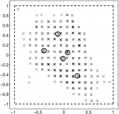
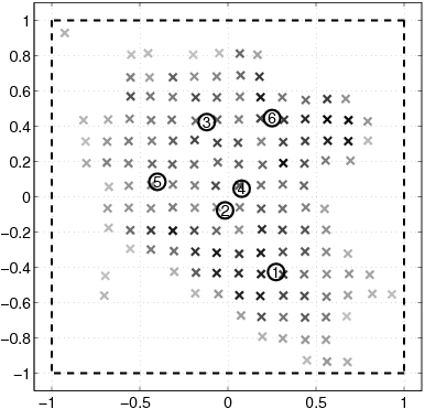
X	Set of all customers.
[(x)\vec]	Location of one customer.
m_[(x)\vec]	Weight of customer [(x)\vec].
l	Library size.
d_j	Popularity of object j.
n	Number of nodes.
[(n)\vec]_i	Location of node i.
l_i	Total resources of node i.
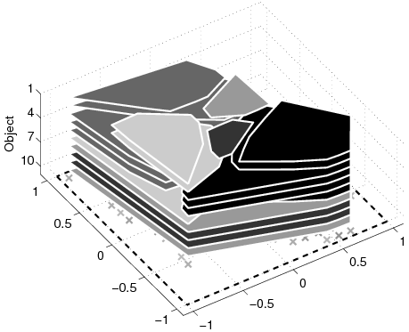
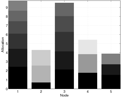
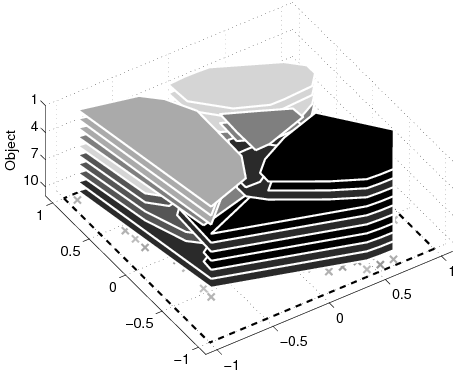
L_ij	Allocation for object j in node i.
C_[(x)\vec]i	communication cost between customer [(x)\vec] and node i.
p_[(x)\vec]ij	Assignment of customer [(x)\vec] to node i for object j.
m	Total weight of the customers.
L	Minimum allocatable resource.
D_ij	Demand in node i for object j.
c	Total number of cached files.
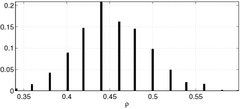
r	Utilization of the caching strategy.
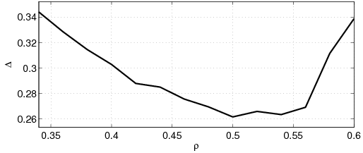
D	Communication cost.
[^(D)]	Fuzzy objective function.
l_j^*	Allocation for object j in the entire network.
j_ij	Mediator variable defined in (23).
w_ij	Mediator variable defined in (31).
y_[(x)\vec]i	Mediator variable defined in (34).

3.1 Problem Statement

Assume that there are N customers, given as the set X. In the model developed in this paper, we look at the problem in the large scale. Thus, the system is assumed to be in a steady state and each customer is assigned a weight, where m_[(x)\vec] > 0 shows the relative utilization of this user. It is clear that setting all m_[(x)\vec] equal to a constant gives a problem in which all customers are equally important. Whereas, we use this more general model, because in this way we can deal with aggregation more efficiently. This idea is adopted from measuring traffic intensity in terms of Erlangs [84] (see [85] for an example in another field). Knowing that m_[(x)\vec]=1 indicates a continuously active customer, we also tolerate m_[(x)\vec] > 1 as a customer which demands more than one video file at a time, for example an apartment building.

The central problem dealt with here, is designing the network which gives all customers access to a library of video files, which we assume includes l items. Several research projects have shown that the distribution of demands for different video files is well-approximated by the Zipf model [24]. In this model, the demand frequency for the j-th video file is given by d_j=cj^-a, where c is a normalization constant. A reasonable approximation for a is given to be 0.729 [24]. See [86,87] for more comprehensive reviews and details.

For practical reasons, including computational efficiency, we are not interested in looking at independent video files. So, we assume that the library includes ul video files bundled into l chunks of u video files. Hence, we have a library of l same-sized objects where,

d_j=

uj
å
j¢=u(j-1)+1

j¢^-a

ul
å
j¢=1

j¢^-a

, 1 £ j £ l,

(1)

is the demand frequency of the j-th object. However, note that the algorithm proposed in this paper is independent of the model for d_js.

The contents of the library will be cached in n nodes. The geometric location of these nodes, with the i-th node denoted as [(n)\vec]_i, and their contents are other unknowns of the problem. As the VoD service highly demands a one-by-one connection [3,1], using the definition of m_[(x)\vec], we denote the total resources of the i-th node as l_i. We assume that this value is based upon a solution to the VoD network design given by a hypothetical algorithm. If for example l_i is five, it means that the respective node can serve a set, [(X)\tilde], of customers which sum to five (å_{[(x)\vec] Î [(X)\tilde]}m_[(x)\vec]=5), simultaneously. Demands made from the i-th node, can potentially be for any of the l objects. Here, we do a steady-state analysis, by assuming that for any object j, the i-th node allocates a fixed amount of its resources to it, which we denote by L_ij. This portion can be zero if that object is not cached in that particular node. In this way we have,

l_i=

l
å
j=1

d_jL_ij, "i.

(2)

From this point on, L_ijs and l_is are only used in visualizations. We emphasize that neither l_is nor L_ijs are known prior to solving the problem. In fact, l_is are calculated based on L_ijs, which are themselves among the decision variables.

While a node should manage its bandwidth, it should also deliberately decide which objects it will be caching, namely, for the i-th node, how many L_ijs are non-zero. The traditional way of embedding this aspect in the optimization problem is to add different terms for communication cost and storage cost into the objective function (for example see [3]). That approach leads to an objective function which includes two terms, making further derivations harder. In this paper, we propose a different method.

Imposing no limitation on the number of non-zero L_ijs, the optimal network will tend to cache every object in every node. This is identical to having l=1 and contradicts the goal behind slicing the library. Returning to the definition of L_ij, our demand is to have either L_ij=0 or a "big" L_ij. This means, if the j-th object is cached in a node, then there should certainly be a reasonable demand for it. For this goal, we define the value of L, as the minimum demand for an object at a node which justifies caching it there. Doing so, we add implicit concern over optimality of storage to the optimization problem. This is carried out through implicit comparison of d_jL_ij with L to decide if the j-th object should be cached in the i-th node, or not.

Assume that the customer [(x)\vec] demands the j-th object which is then supplied from the i-th node. The net cost of this transaction is modeled as C_[(x)\vec]i, and is assumed to be independent of the object which is transmitted. The simplest assumption is that C_[(x)\vec]i is given as a lookup-table, for one set of nodes. In this way, the algorithm proposed here cannot optimize the location of the nodes, while the rest of the algorithm will still work. As a better formulation, we consider the case where C_[(x)\vec]i is a function of the Euclidean distance between [(x)\vec] and [(n)\vec]_i. Here, we focus on the cost model defined as,

C_[(x)\vec]i=C||

||^m_d, m_d ³ 1,

(3)

where C is a constant which is ignored in the rest of this analysis.

Focusing on a particular customer, [(x)\vec], this customer will demand access to all objects, with different probabilities. Assuming that this customer demands the j-th object for j=1,¼,l from the k_j-th node, where 1 £ k_j £ n, the expected cost of providing one object, any object, to this customer equals,

D_[(x)\vec]=

l
å
j=1

d_jC_{[(x)\vec]k_j}.

(4)

To simplify (4), we define p_[(x)\vec]ij Î {0,1}, where, p_[(x)\vec]ij is one iff [(x)\vec] asks the node i for the j-th object. So,

n
å
i=1

p_[(x)\vec]ij=1, "

, j.

(5)

Now, we can rewrite (4) as,

D_[(x)\vec]=

l
å
j=1

æ
è

d_j

n
å
i=1

C_[(x)\vec]ip_[(x)\vec]ij

ö
ø

(6)

Including weights of the customers, the expected cost of serving one demand from any customer equals,

D =

å
[(x)\vec] Î X

æ
è

m_[(x)\vec]

l
å
j=1

æ
è

d_j

n
å
i=1

C_[(x)\vec]ip_[(x)\vec]ij

ö
ø

(7)

Here,

m =

å
[(x)\vec] Î X

m_[(x)\vec].

(8)

Following the definition of L_ij, as allocation at node i for the j-th object, we define D_ij as the demand in the i-th node for the j-th object. Thus, we have,

D_ij=

å
[(x)\vec] Î X

m_[(x)\vec]p_[(x)\vec]ij,

(9)

Note that in a stable network, allocation and demand are identical. Thus, we should have,

L_ij=D_ij, "i,j.

(10)

Satisfaction of this equation not only depends on L_ijs, but also depends on p_[(x)\vec]ijs, through D_ijs. While (9) yields,

n
å
i=1

D_ij=m, "j,

(11)

accompanied by (10), it also gives,

n
å
i=1

L_ij=m, "j.

(12)

At this stage, the optimization problem is defined as minimizing,

D =

å
[(x)\vec] Î X

æ
è

m_[(x)\vec]

l
å
j=1

æ
è

d_j

n
å
i=1

C_[(x)\vec]ip_[(x)\vec]ij

ö
ø

(13)

subject to,

n
å
i=1

p_[(x)\vec]ij=1, "

, j,

(14)

L_ij=

å
[(x)\vec] Î X

m_[(x)\vec]p_[(x)\vec]ij, "i,j,

(15)

(L_ij=0) or (d_jL_ij ³ L), "i,j.

(16)

Here, p_[(x)\vec]ijs, L_ijs, and [(n)\vec]_is are the decision variables. While this optimization problem is defined as minimizing D, it is still important to know how many objects are totally cached. To measure this phenomenon, we define the value of c as the number of L_ijs which are nonzero. As two extreme solutions, consider the case in which every object is cached in every node and the case in which no node is caching anything, except for one node, which caches every object. The associated c values for these solutions are nl and l, respectively. Note that at least the second case is a locally optimal solution. Also, that case can happen with a set of nodes caching all the objects, with each object being cached only by one node and all nodes residing on the same exact physical location. This solution is also locally optimal and gives c=l. As analysis shows that l £ c £ nl, and to be independent of n and l, we define the utilization of the caching strategy as r = [c/nl]. Accordingly, while we mainly focus on minimizing D, we also want to keep the value of r small. This is partly done by the minimum bound on non-zero L_ijs. We return to the value of c and r in Section III-C.

In Section III-B, we rewrite the problem defined in this section as a mixed integer linear programming (MILP) problem, which will be translated into the General Algebraic Modeling System (GAMS) and solved using the NEOS server [88,89,90]. Then, in Section III-C, we reformulate the problem, using an approximation to relax one of the constraints, and then transfer it into fuzzy domain.

3.2 MILP Formulation

To write the optimization problem given at the end of Section III-A as a MILP problem, we use (10) and (9) and rewrite (16) as,

d_j

å
[(x)\vec] Î X

m_[(x)\vec]p_[(x)\vec]ij £ mq_ij, "i,j,

(17)

d_j

å
[(x)\vec] Î X

m_[(x)\vec]p_[(x)\vec]ij+m(1-q_ij) ³ L, "i,j.

(18)

Here, q_ijs are unknown binary decision variables. These two constraints, accompanied by (14), and the objective function given in (13) constitute the MILP optimization problem. The decision variables of this optimization problem are p_[(x)\vec]ijs, q_ijs, and [(n)\vec]_is. Note that, q_ij=1 iff the j-th object is cached in the i-th node. Similarly, substituting q_ij=0 in (17) yields p_[(x)\vec]ij=0 for all [(x)\vec]s and the given i and j. After setting up this problem as a GAMS model, we use the BDMLP solver. BDMLP is a simplex-based solver which is designed for small and medium-sized problems [91]. Using this general-purpose solver we find a typical solution a blind optimizer will give to this problem. This solution will then be used to assess the efficiency of the proposed algorithm.

3.3 Proposed Formulation

The optimization problem given at the end of Section III-A is not analytically attractive, because it includes the binary decision variables of p_[(x)\vec]ijs. The two available choices for the L_ijs also add to the difficulty of analytically tackling this problem. In the following parts of this section, we give an approximate form of this optimization problem, which resembles fuzzy clustering problems, and is analytically manageable. First, we relax (16) by adding L_ijs as controlling weights to the objective function. The weights are designed in a way that we can exclude (16) from the constraints but still satisfy an approximate form of (10) defined as,

L_ij @ D_ij, "i,j.

(19)

In addition, to control allocation of objects, we add (12) as a constraint. We then translate the objective function into a fuzzy representation.

Looking at (7), we write the cost of serving the j-th object to all customers as,

D_j=

å
[(x)\vec] Î X

æ
è

m_[(x)\vec]

n
å
i=1

C_[(x)\vec]ip_[(x)\vec]ij

ö
ø

(20)

This objective function, accompanied by the constraint given in (5), is very well known as described below. Assuming m_d=2 and m_[(x)\vec] º 1, this is a simple Weber problem. As briefly reviewed in Section II-F, this problem is called HCM in clustering theory. The name HCM is selected because we are doing a binary (hard) clustering of a given set of points into spherical clusters which are identified by their means (C-means). This problem has been known for a long time in the literature and several generalizations of it exist. A straight-forward generalization is the introduction of weights into the problem (see [92,93] for example). This means that different data points are differently important. As also mentioned in Section II-F, fuzzy clustering is a heuristic extension to this problem, in which p_[(x)\vec]ij Î {0,1} is replaced with p_[(x)\vec]ij Î [0,1] and (20) is rewritten as,

å
[(x)\vec] Î X

æ
è

m_[(x)\vec]

n
å
i=1

C_[(x)\vec]ip_[(x)\vec]ij^m

ö
ø

(21)

for m close to one. As mentioned in Section II-F, this problem is called FCM and experimental analysis during the last two decades has shown that this extension is beneficial in different problems in coding and pattern recognition [94]. Here, we choose the same approach and give a fuzzy version of (7) by rewriting it as,

å
[(x)\vec] Î X

æ
è

m_[(x)\vec]

l
å
j=1

æ
è

d_j

n
å
i=1

C_[(x)\vec]ip_[(x)\vec]ij^m

ö
ø

(22)

where (5) is still in place and p_[(x)\vec]ij Î [0,1]. Here, m > 1 is the fuzziness [58]. It is known that, generally, as m tends to 1⁺, the fuzziness of p_[(x)\vec]ijs reduces [68]. In this way, we will have p_[(x)\vec]ij Î [0,d]È[1-d,1] for a small d. While this is the classical approach also used in FCM [59], we further use relabeling [66] to convert the minimally fuzzy p_[(x)\vec]ijs into members of {0,1} by picking the most likely connection for each customer and each object. Note that, we still need to incorporate storage cost into the objective function.

As mentioned earlier, L^-1d_jL_ij is expected to be either zero or bigger than one. In the first case, no customer is expected to rely on the i-th node for the j-th object. This is a two-choice constraint which makes the objective function discontinuous and hence hard to work with. Also, it adds an extra constraint to the optimization problem and makes the application of FCM-style optimization hard. To solve these problems, we define the term j_ij as,

j_ij=1+

æ
è

d_jL_ij

ö
ø

-k

(23)

Here, k is a fixed power, with default values over 10. Now, as L_ij tends to zero, j_ij approaches infinity. On the other hand, j_ij tends to one for d_jL_ij ³ L. We use this term to add a force to the objective function to carry out three goals. Namely, it helps satisfy (19), it forces small d_jL_ijs to become zero, and it becomes transparent when the solution converges. We will discuss these points in detail in the next paragraph.

Using j_ijs, we rewrite (22) as,

å
[(x)\vec] Î X

æ
è

m_[(x)\vec]

l
å
j=1

æ
è

d_j

n
å
i=1

C_[(x)\vec]ip_[(x)\vec]ij^mj_ij

ö
ø

(24)

Note that j_ij is a decreasing function of L_ij. Thus, if L_ij becomes small, j_ij tends to a very large value. Then, as [^(D)] is minimized, non-zero p_[(x)\vec]ij, for the given i and j, will lead to a big contribution to [^(D)] and thus will not happen in the maximizer. Thus, the introduction of j_ij into (24) has the effect of refraining customers from requesting objects from nodes in which they are not cached, or where little resources are allocated to them. In a similar way, for large L_ijs, j_ij becomes small and thus more p_[(x)\vec]ijs will be attracted to the respective node. This will result in increasing D_ij. In a similar way, smaller L_ijs are likely to result in smaller D_ijs. This is a balancing force which allows (19) to be satisfied. On the other hand, when L_ij becomes small and hence no p_[(x)\vec]ij is big, then if this L_ij becomes zero, it will result in other L_i¢js benefiting from (12) and growing larger. This will result in smaller j_i¢js, eventually leading to a smaller [^(D)]. Thus, the j_ij weights are also beneficial in pushing small L_ijs towards zero. Finally, for active L_ijs, meaning those which are not zero, j_ij is close to one. If we can also have minimally fuzzy p_[(x)\vec]ijs, for which p_[(x)\vec]ij^m @ p_[(x)\vec]ij, then [^(D)] will be approximately equal to D. Thus, j_ijs will be transparent and minimizing (24) will eventually result in minimizing (7). In Section IV we show how these tendencies act in a real problem. We also show how to move from (19) to (10).

To summarize, the VoD network design problem is approximated as minimizing,

å
[(x)\vec] Î X

æ
è

m_[(x)\vec]

l
å
j=1

æ
è

d_j

n
å
i=1

C_[(x)\vec]ip_[(x)\vec]ij^mj_ij

ö
ø

(25)

subject to,

n
å
i=1

p_[(x)\vec]ij=1, "

, j,

(26)

n
å
i=1

L_ij=m, "j.

(27)

This formulation is one of the main contributions of this paper. From this point on, we will work on giving a solution to this optimization problem. To do so, in the next section, we propose an algorithm for finding a local minimizer for this problem.

3.4 Solving the Problem: Single Trial

Remembering the FCM methodology, we use Lagrange Multipliers to rewrite the objective function as [95],

F =

l
å
j=1

å
[(x)\vec] Î X

l_[(x)\vec]j

æ
è

n
å
i=1

p_[(x)\vec]ij-1

ö
ø

l
å
j=1

g_j

æ
è

n
å
i=1

L_ij-m

ö
ø

(28)

Setting [(¶F)/(¶p_[(x)\vec]ij)]=0 and using (5) we have,

p_[(x)\vec]ij=

(C_[(x)\vec]ij_ij)^-[1/(m-1)]

n
å
i¢=1

(C_[(x)\vec]i¢j_i¢j)^-[1/(m-1)]

(29)

Also, deriving [(¶F)/(¶L_ij)] and equating it to zero and then using (12) we will have,

L_ij=m

w_ij^[1/(k+1)]

n
å
i¢=1

w_i¢j^[1/(k+1)]

(30)

Here,

w_ij=

å
[(x)\vec] Î X

m_[(x)\vec]C_[(x)\vec]ip_[(x)\vec]ij^m.

(31)

To optimize F in terms of [(n)\vec]_is, we will look at the case when m_d is 2 and when it is not independently. When m_d=2, using the equation,

¶C_[(x)\vec]i

æ
è

ö
ø

(32)

we have,

å
[(x)\vec] Î X

y_[(x)\vec]i

å
[(x)\vec] Î X

y_[(x)\vec]i

(33)

Here,

y_[(x)\vec]i=m_[(x)\vec]

l
å
j=1

d_jj_ijp_[(x)\vec]ij^m.

(34)

When m_d is not two, we cannot use the formulation given in (33) for finding [(n)\vec]_i [96]. Thus, we utilize a method similar to the Weiszfeld approach [70], except for the fact that the original Weiszfeld method only works for m_d=1 [40,82]. Using (3) we have [97],

¶C_[(x)\vec]i

=m_d||

||^m_d-2

æ
è

ö
ø

(35)

Hence, equating [(¶F)/(¶[(n)\vec]_i)] with zero we have,

å
[(x)\vec] Î X

y_[(x)\vec]i||

||^m_d-2

å
[(x)\vec] Î X

y_[(x)\vec]i||

||^m_d-2

(36)

Now, we use the fixed point method. To do this, we use the initialization vector of,

0
i

å
[(x)\vec] Î X

y_[(x)\vec]i

å
[(x)\vec] Î X

y_[(x)\vec]i

(37)

This idea is adopted from the similar initialization in the Weiszfeld method [48]. Now, we define,

t+1
i

å
[(x)\vec] Î X

y_[(x)\vec]i||

t
i

||^m_d-2

å
[(x)\vec] Î X

y_[(x)\vec]i||

t
i

||^m_d-2

(38)

The computation of (38) is performed for each value of i until ||[(n)\vec]_i^t+1-[(n)\vec]_i^t|| becomes less than a specified threshold. Note that while here we have used the power model shown in (3), similar approach is applicable to many other formulations, at least to many of those that satisfy,

C_[(x)\vec]i=C

æ
è

||²

ö
ø

(39)

for a differentiable function C (see Appendix A).

Here, we have not provided any convergence proof for the iteration depicted in (38). However, we do know that for m_d=2, the iteration changes into a one-step weighted average calculation, shown in (33). Also, it is proved that for m_d=1 the algorithm converges to a unique point [98], in a linear fashion [40]. Numerous experiments show that for the case of m_d ³ 1, the algorithm converges. Based on this observation, we conjecture that for m_d ³ 1 the iteration given in (38) converges. Providing a proof for this conjecture is still an open problem. However, in Appendix B, we give a theorem which shows why m_d ³ 1 is important.

The approach adopted here, is based on the basic Weiszfeld method. Whereas, there are methods for accelerated Weiszfeld which increase the convergence speed (for example see [99,37]). We do not address the acceleration methods in this paper.

fVoD Algorithm

Inputs:	n: Number of nodes.
	l: Number of objects.
	X: Set of all customers.
	m_[(x)\vec]: Weights of the customers.
	d_j: Objects' demands.
	m_d: Power in (3).
	m: Fuzziness.
	k: Power in (23).

Outputs:	L_ij: Allocation pattern.
	[(n)\vec]_i: Nodes' locations.
	p_[(x)\vec]ij: Membership values.
	D: Value of the objective function.

1- [^(D)]=¥

2- Randomly produce [(n)\vec]_is.

3- Randomly produce L_ijs which comply with (12).

4- Use (29) to produce p_[(x)\vec]ijs.

5- Use (30) to produce L_ijs.

6- if m_d=2, use (33) to produce [(n)\vec]_is.

7- if m_d ¹ 2, use (37) and (38) to produce [(n)\vec]_is.

8- [^(D)]^o=[^(D)]

.9- Use (24) to produce [^(D)].

10- If [^(D)]^-1|[^(D)]-[^(D)]^o| > e, go to 4.

11- Calculate D_ijs using (9).

12- L_ij=D_ij.

Figure 2: Details of the algorithm fVoD. Everywhere j=1,¼,l, i=1,¼,n, and [(x)\vec] Î X. Here, e is the precision which we select to be 10^-4 for our experiments.

Using these results, in an FCM-style iterative algorithm, we can produce a locally optimal solution. However, note that this solution is only likely to satisfy (19), and not (10). Here, we propose a method to alter the solution to produce one which does satisfy (10). Having calculated the optimal p_[(x)\vec]ijs, we can calculate D_ijs, using (9). According to (11), if we replace all L_ijs with the respective D_ijs, Equation (27) will be intact. However, this manipulation might results in an increase in c, because of a previous unbalance in allocation-demand which has resulted in a spurious small utilization. Thus, we argue that the new value of c shows the actual number of cached objects. Nevertheless, this manipulation does not affect D.

Utilizing the results derived in this section, we propose the algorithm depicted in Figure 2 to find a potential locally optimal network design. We call this algorithm Fuzzy Video on Demand Network Design or fVoD.

As we do not have any proof for the convexity, or concavity, of [^(D)] [100], we cannot make any argument about the possibility of fVoD not being trapped in a local minimum. In fact, in [46], the authors show the example of a similar problem which has 50 customers and 61 local minimums (also see [101]). However, we do know that fVoD does converge, because at any iteration the produced solution is better than what was worked out in the previous one (here we are assuming that we have proof for the convergence of (38) for m_d Î (1,¥)-{2}). So, we can safely say that fVoD does find a locally optimal solution, whereas, the outcome is dominantly affected by the initial choice of [(n)\vec]_is and L_ijs [102]. We use this unrepeatability to propose the fVoD^m algorithm in the next section. Before that, an analysis of the computational cost of the proposed algorithm and a note about allocation-related variables are given below.

Define the variables w and u as the number of iterations of the Weiszfeld-style calculation given in (38) and fVoD, before they converge, respectively. According to experimental results, maximum typical values for these parameters are w=10 and u=25, when N=50, n=5, and l=10. Now, the approximate cost of fVoD is 15Nnlu flops and 15Nnlu+9Nnwu flops for the cases of m_d=2 and m_d ¹ 2, respectively.

While L_ijs are the decision variables in the proposed optimization problem, they can also be used in deriving other measures such as allocation in any node or for any object. In this way, in addition to allocation at each node, which is defined in (2), we define allocation for the j-th object in the entire network as,

l_j^*=d_j

n
å
i=1

L_ij.

(40)

Accompanied by l_i, these measures will be used in visualizing a potential solution.

3.5 Solving the Problem: Searching For a Better Solution

As mentioned in Section III-D, the solution produced by fVoD may only be locally optimal. However, we do know that running multiple instances of fVoD produces potentially different solutions. Thus, we propose to run fVoD for T independent times. Let's call the i-th solution S_i, represented by the pair (D_i,r_i). A practical way for dealing with the existence of two optimality criteria, D_i and r_i, is to devise a function of them as the total optimality criterion and then to pick the best solution based on that. Note that, here, D_i and r_i directly represent the communication cost and the storage cost, respectively. While seeming simple to implement, this approach demands a cost model which can address the cost of communication and storage at the same time. For this purpose, a reasonable idea is to calculate a linear combination of D_i and r_i, with weights estimated from the actual cost of the equipments. However, we refrain from following this approach, because we do not have these figures. To deal with this problem, we filter out the solutions which demand too much storage space. Therefore, we pick a value of r₀ and then from the set of solutions which satisfy r_i £ r₀, we pick the one which corresponds to the least D. We call this algorithm fVoD^m. Note that the more computational resources are given to the fVoD^m algorithm, the more optimal results it will produce. This scalability is important for procedures designed for real applications.

3.6 Application Scenarios

In Sections III-D, the general structure of the fVoD algorithm was presented. Also, in Section III-E a heuristic technique was devised to find more optimal solutions. In this section, we refer to the practical framework in which the proposed algorithms can be utilized. First, the minimal and the maximal scenarios are discussed.

The minimal scenario in which fVoD can be implemented is as a part in a bigger human-directed design process. In this way, as a designer works on the VoD network, the relationships given in Section III-C can be used to optimize one aspect of the design. For example, knowing the placement of the nodes and the caching pattern, we can use (29) to calculate the optimal assignment. Also, knowing the nodes' locations and the assignment, one can use (30) to optimize caching. Similarly, knowing caching and assignment, the right combination of (33) or (37) and (38), will give the optimal location for the nodes.

The maximal scenario is the assumption that fVoD is responsible for designing the whole network, including locating the nodes. This hypothetical scenario can be carried out by fVoD. However, it should be emphasized that this scenario is mostly of theoretical interest, because the problem VoD service providers are more concerned with is the growth and maintenance of available networks. These concerns are addressed by fVoD through a slight change in the algorithm depicted in Figure 2. As discussed in Section III-D, the essence of fVoD is local improvement of a design. Thus, by jumping over recalculation of L_ijs, [(n)\vec]_is, or p_[(x)\vec]ijs, whichever and wherever necessary, these variables will be made fixed in the entire design. In this way, we can optimize only a part of the design.

Here, as an example, we discuss the two cases of staged network growth and caching optimization. In both scenarios, we define the values q₁,¼,q_n Î {0,1}, where q_i=1 means the location of the i-th node cannot change. The consecutive changes in the algorithm depicted in Figure 2 would be rewriting Lines 6 and 7 as, "¼ to produce [(n)\vec]_i for all q_i=0". Also, in Line 2, only those [(n)\vec]_is for which q_i is zero will be randomized. In the new version of fVoD, adding n₁ nodes to a network with n₂ available nodes will be carried out through using q₁,¼,q_n₁+n₂, where,

q_i=

ì
ï
í
ï
î

i £ n₁

otherwise

(41)

Here, the initial values for [(n)\vec]_i, i > n₁ come from the available nodes. Similarly, recalculating the optimal caching and assignment strategy for an available network will be carried out through using an all-one q sequence, where no [(n)\vec]_i is randomized. In Section IV, these scenarios will be looked into using sample problems.

4 Experimental Results

The proposed algorithm is developed in MATLAB 7.0.4 on a PIV 3.00GHZ with 1GB of RAM. In this section, we analyze three scenarios and show the outcome of the algorithm in each one of them. First, we assume that a population is given and that the algorithm should design the whole network. This scenario is discussed in Section IV-A. Then, in Section IV-B, we assume that the underlying geographical area has expanded and thus a new node should be added to the network. Finally, Section IV-C assumes that the pattern of population has changed and hence the caching policy should be re-optimized. In each scenario, the contributions of the proposed algorithm are discussed.

To produce the aggregated population, in each case, a gray-scale image is used as the population density map. This image is sliced into blocks and the average color and the weighted central point for each block are calculated. Rejecting those blocks which exhibit average color less then a minimum threshold, the central points are stored in a set, each accompanied by the respective weight, i.e. the average color.

4.1 First Scenario: Complete Design


(a)	(b)

Figure 3: Population density in the first scenario. (a) Input population map. (b) Aggregated customers.

The image used in this scenario is the one shown in Figure 3-a, from which N=133 aggregated customers, as shown in Figure 3-b, are extracted. Using these customers, the problem is defined as locating n=5 nodes to cache l=10 objects. Here, we select the power in the cost model to be m_d=1.3. Also, the objects' demand frequencies are calculated based on a Zipf(0.729) distribution.


(a)	(b)

Figure 4: VoD network designed by BDMLP in the first scenario. (a) Location of the nodes. (b) 3-D representation of the network.

Using the BDMLP solver, this problem is solved in six minutes on a PIV 2.53GHz with 512MB of RAM. The result is a solution for which D = 0.463 and r = 0.2. Figure 4 shows this solution. As seen in Figure 4-a, the first and the second nodes are located on the same physical point. These two nodes make a hyper-node which caches each object once and only once.

To give a visual representation of the resulting network, we draw a three dimensional graph with l layers, in which each layer shows the connection pattern for one object. To give an intelligible visualization of the connections, in each layer the convex hull of all the customers which access the same object through the same node is drawn. This is performed in Figure 4-b for the solution generated by BDMLP, and in other figures used for visualizing other solutions hereafter. In this figure, each shade indicates one node. Here, clearly, every connection originates from the hyper-node.

Attempting to optimize this solution using subsets of variables, it appears to be a locally optimal solution to the approximate formulation. However, note that, this solution neglects the main reason behind slicing the library into objects. We will also see that the proposed algorithm is able to produce a solution in which the communication cost is considerably lower.

To apply the proposed method, the values of parameters are selected as m=1.1, k=15, and T=1000. Also, to produce a reasonable value of L, ¹/₂d_lm is used. Here, d_lm represents the maximum possible value of d_jL_ij for j=l, and thus the maximum bound for L. Using these parameters, the fVoD^m algorithm takes about ten minutes to run. Note that except for the set of customers and n, other scenarios use the same values of parameters, where L is independently calculated in each case.

In this scenario, the fVoD^m algorithm produces 1000 potential solutions, for which we have, D_i Î [0.262,0.521] and r_i Î [0.34,0.60]. Figure 5-a shows the least D for each value of r in these solutions. As seen here, as r approaches half, the cost decreases. The increase of D for r > 0.5 relates to locally optimal solutions which cache very inefficiently. To describe the unexpectable rise in the cost for these values of r, we refer to the histogram of r, shown in Figure 5-b. As seen here, there are very few solutions for which r > 0.53. The increased least available cost for this range of r is then because less local solutions in this range have been examined.


(a)	(b)

Figure 5: Analysis of the solutions produced by the proposed algorithm for the first scenario. (a) Least D for each value of r. (b) Histogram of values of r.

Here, we select the utilization threshold to be r₀=0.40. After the filtering stage 849 solutions remain, from which fVoD^m retrieves one for which D = 0.303 and r = 0.4. This solution is comprehensively analyzed in the next parts of this section.


(a)	(b)

Figure 6: VoD network designed by the proposed algorithm in the first scenario. (a) Location of the nodes. (b) 3-D representation of the network.

Figure 6-a shows the location of the nodes in this solution. Looking at the structure of the network, shown in Figure 6-b, we observe that the first objects are cached in many nodes, while the last ones are each only stored in one node. This was expected, because the criterion for caching an object is the value of d_jL_ij. Thus, for the last objects, which have smaller d_js, L_ij should be big, resulting in less number of L_ijs being non-zero (see (12)).


(a)	(b)

Figure 7: Aggregate allocation for nodes and objects in the solution to the first scenario. (a) Allocation in each node. Different colors show different objects. (b) Allocation for each object. Different colors show different nodes.

Using L_ijs, Figure 7-a shows the aggregate allocation at each node (l_i). Here, different colors denote different objects. Similarly, Figures 7-b shows the aggregate allocation for different objects in the entire network (l_j^*). Here, different colors indicate different nodes. We can use these charts to show how the caching strategy changes in the network, under different circumstances.


(a)	(b)

(c)	(d)

Figure 8: Investigating the solution to the first scenario. (a) Histogram of p_[(x)\vec]ijs. (b) Histogram of active j_ijs. (b) Number of objects cached in each node. (d) Number of nodes in which each object is cached. In (c) and (d), the solid lines show the actual values while the dashed lines show the maximum possible ones.

Finally, we look at some internal variables (see Figure 8). Figure 8-a shows the histogram of p_[(x)\vec]ijs. As seen here, assignment is minimally fuzzy. In fact, 96% of p_[(x)\vec]ijs are either less than 0.03 or more than 0.97. Figure 8-b shows the histogram of the active j_ijs, showing their closeness to one. In fact, active j_ijs vary between 1.14 and 1, the ideal value. Furthermore, the solid line in Figure 8-c shows the number of objects cached in each node. Here, the dashed line shows the maximum value, l. Thus, in the network designed here, in average, each node has cached 40% of the library (r = 0.4). Looking at the solid line in Figure 8-d, we see the number of nodes in which each object is cached. Here, the dashed line shows the maximum possible values, min{L^-1d_jm,n}. This figure shows that while the first object is cached in every node, the four last objects are only cached in one node, each.

Comparing the solution rendered by the proposed method and the one produced by BDMLP, we observe that with a similar computational complexity the proposed algorithm cuts the cost at about 35%. Thus, for the next scenarios, we only analyze the results of the proposed algorithm. Note that the intrinsic level of flexibility which is present in fVoD is not achiveable in a general optimization problem, unless the problem is reorganized to separate known parameters from decision variables, in every case, independently.

The charts shown in Figures 7 and 8 show the solution from different perspectives. These visualizations are helpful in looking into details of a solution and finding probable shortcomings. To save space, we do not give detailed figures for the two next scenarios and only the structure of the network and the values of D and r are discussed.

4.2 Second Scenario: Adding One Node


(a)	(b)

Figure 9: Population density in the second scenario. (a) Input population map. (b) Aggregated customers.

As the underlying population pattern changes, the efficiency of the VoD system designed based on that pattern may decrease. This is one of the main challenges the VoD service providers are faced with. In the second scenario, we assume that it is necessary for a VoD network, here the network designed in Section IV-A, to add a new node to the system, because of a newly added region to its coverage area. Subsequently, this change will result in recalculation of the caching strategy for all nodes plus a new assignment.

Figure 10: Aggregate allocation for nodes in the solution to the first scenario after it is optimized by the proposed algorithm to fit the second scenario. Different colors show different objects.

The population density map for this scenario is shown in Figure 9-a, with the new region added in the right. Using this map, N=144 aggregated customers, as shown in Figure 9-b, are extracted. To have numerical figures to describe the situation before optimization is carried out, we use a minimal version of fVoD to recalculate the optimal assignment, using (29). This also results in a new caching strategy shown in Figure 10. Comparing this figure with Figure 7-a shows the change in allocation, caused by fVoD, to fit the available network to the new circumstances. Here, we have D = 0.337 and r = 0.4. This means that the application of the previous design for the new population increases the cost by 11%. Now, we use fVoD^m to locate the new node and also to recalculate the caching strategy and the assignment.


(a)	(b)

Figure 11: VoD network designed by the proposed algorithm in the second scenario. (a) Location of the nodes. (b) 3-D representation of the network.

To do so, we use the q_i sequence defined as (0,1,1,1,1,1), meaning one extra node is needed while the five available ones cannot be displaced. The output of fVoD^m, after ten minutes of calculation, is a solution for which D = 0.308 and r = 0.4. These figures show that the application of fVoD^m has caused about 10% decrease in the communication cost. Comparing this figure with the cost in the first scenario, the addition of the new node has compensated for the newly added region and the cost is only less than 2% more in the new solution. Figure 11 shows this solution. As requested, five available nodes are not displaced, while their cached content is recalculated. Also, as anticipated, the new node is located close to the newly added population. These results should now be investigated by a superviser, to decide whether the costs of erecting a new node justifies the reduction in costs.

4.3 Third Scenario: Caching Optimization


(a)	(b)

Figure 12: Population density in the third scenario. (a) Input population map. (b) Aggregated customers.

Section IV-B discussed the case in which the change in population was to be dealt with by adding a new node. Here, we analyze a less severe situation, where the change in population does not justify addition of a new node, according to a hypothetical expert's idea. Thus, the algorithm needs to only recalculate the optimal caching and assignment strategies. Figure 12-a shows the new population map, from which 150 customers are extracted, as shown in Figure 12-b.

To find the current costs, we use a minimal fVoD to recalculate the optimal assignment, using the known nodes and their respective content. This situation results in D = 0.323 and r = 0.37, showing about 5% increase in the cost.


(a)	(b)

Figure 13: VoD network designed by the proposed algorithm in the third scenario. (a) Location of the nodes. (b) 3-D representation of the network.

Now, using the q_i sequence defined as (1,1,1,1,1,1), the fVoD^m algorithm is used to optimize both the caching strategy and the assignment. Taking about ten minutes of calculation, a solution is rendered in which D = 0.319 and r = 0.4, showing 1% decrease in the cost. Again, we see that fVoD^m is able to produce a solution in which cost is reduced. The new solution is shown in Figure 13.

Thus, it was shown that the proposed algorithm, and its minimal implementations, are able to address a vast group of optimization requests in a VoD network. These demands vary from recalculating the optimal assignment or caching to designing the whole network. A major point about the proposed algorithm is that here we are using the same algorithm for different optimization tasks. Also, the proposed algorithm is designed in a way that the more computational resources are given to it, the more optimal its output will get. Therefore, the algorithm can be used as a quick effort for finding a slightly better solution or a time consuming more global search. Note that while we did not give a mathematical proof for the convergence of the generalized Weiszfeld, it is utilized in the experimental results discussed in this paper for about half a million times and it has converged in every single utilization. Empirically, based on the experiments reported on here, it appears to be a reasonable conjecture that the convergence of the proposed method could be guaranteed, although we have no proof for it.

5 Conclusions

In this paper, we focused on the Video-on-Demand (VoD) network design problem. Using concepts and tools available in signal coding, an optimization problem was developed which was shown to minimize the communication cost in a VoD network. Also, weights were added to the cost function to implicitly control storage cost. According to the zero-one property of the original problem, the objective function included binary variables, which made it mathematically hard to work with. So, looking back at fuzzy clustering, the problem was transferred into fuzzy domain. The transformation was carried out in a way that the fuzziness of the solution was guaranteed to be acceptably low. Then, a method was proposed to produce a locally optimal solution to the proposed objective function, using an iterative three-stage algorithm. Benefiting from the fact that the proposed algorithm is unrepeatable, another algorithm was proposed to produce a set of potential solutions and then to heuristically pick a proper one of them. Then, defining three main scenarios, the application of the proposed algorithm was discussed. The first scenario investigated the hypothetical application of the proposed method in designing the whole network. The two other scenarios discussed adding a new node to the network and recalculating caching and assignment, both because of changes in the population density map. In all cases, the contributions of the proposed algorithm were discussed using both numerical measures and also visual representations. Also, the result of the proposed algorithm in the first scenario was compared with that of mixed integer linear programming (MILP). It was shown that MILP traps in a local minimum, in which only one hyper-node serves the whole network. It is worth to mention that the convergence of the proposed algorithm was empirically observed. However, a more general proof for the generalized Weiszfeld method, proposed here, is still needed.

Acknowledgment

The research of Attahiru Sule Alfa is partially supported by a grant from NSERC. The authors appreciate comments by Jeff Rohne on the practical scenarios under which the proposed algorithm can be used. Also, we appreciate the help from NEOS team, especially Jason Sarich. The first author wishes to thank Ms. Azadeh Yadollahi for her encouragement and valuable discussions. We also appreciate the respected anonymous referees for their constructive suggestions.

References

[1]: H. Ma and K. G. Shin, "Multicast video-on-demand services," ACM SIGCOMM Computer Communication Review, vol. 32 (1), pp. 31-43, 2002.
[2]: T. D. Little and D. Venekatesh, "Prospects for interactive video-on-demand," IEEE Multimedia, vol. 1 (3), pp. 14-24, 1994.
[3]: J.-P. Nussbaumer, B. V. Patel, F. Schaffa, and J. P. G. Sterbenz, "Networking requirements for interactive video on demand," IEEE Journal on Selected Areas in Communications, vol. 13 (5), pp. 779-787, 1995.
[4]: T. S. Perry, "The trials and travails of interactive TV," IEEE Spectrum, vol. 33 (4), pp. 22-28, 1996.
[5]: C. Vassilakis, M. Paterakis, and P. Triantafillou, "Video placement and configuration of distributed video servers on cable TV networks," Multimedia Networks, vol. 8, pp. 92-104, 2000.
[6]: J. Segarra and V. Cholvi, "Distribution of video-on-demand in residential networks," in Proceedings of the 8th International Workshop on Interactive Distributed Multimedia Systems, 2001, pp. 50-61.
[7]: R. L. Francis, T. J. Lowe, and A. Tamir, "Demand point aggregation for location models," in Facility Location, Applications and Theory, Z. Drezner and H. W. Hamacher, Eds. Berlin: Springer-Verlag, 2002, pp. 179-205.
[8]: K. Park, K. Lee, S. Park, and H.Lee, "Telecommunication node clustering with node compatibility and network survivability requirements," Management Science, vol. 46 (3), pp. 363-374, 2000.
[9]: K. H. Muralidhar and M. K. Sundareshan, "On the decomposition of large communication networks for hierarchical control implementation," IEEE Transactions on Communications, vol. COM-34 (10), pp. 985-987, 1986.
[10]: Y. G. Saab, "A fast and robust network bisection algorithm," IEEE Transactions on Computers, vol. 44 (7), pp. 903-913, 1995.
[11]: M. Maravalle, B. Simeone, and R. Naldini, "Clustering on trees," Computational Statistics & Data ANalysis, vol. 24, pp. 217-234, 1997.
[12]: V. K. Balakrishnan and C. Moire, Network Optimization. London: Chapman & Hall Mathematics, 5th edition, 1995.
[13]: J. A. M. Pérez, J. M. M. Vega, and J. L. Verdegay, "Fuzzy location problems on networks," Fuzzy Sets and Systems, vol. 142 (3), pp. 393-405, 2004.
[14]: R. K. Ahuja, T. L. Magnanti, and J. B. Orlin, "Network optimization," in Handbook of Applied Optimization, P. M. Paradalos and M. G. C. Resende, Eds. Madison Avenue, New York, New York: Oxford University Press, 2002, pp. 352-363.
[15]: --, Network Flows: Theory, Algorithms, and Applications. NJ: Prentice Hall, 1993.
[16]: F. Glover and D. Klingman, "Network applications in industry and government," AIEE Transactions, vol. 9, pp. 363-376, 1976.
[17]: P. Chardaire and A. Lisser, "Mimum-cost multicommodity flow," in Handbook of Applied Optimization, P. M. Paradalos and M. G. C. Resende, Eds. Madison Avenue, New York, New York: Oxford University Press, 2002, pp. 404-422.
[18]: M. Gerla and L. Kleinrock, "On the topological design of distributed computer networks," IEEE Transactions on Communications, vol. 25 (1), pp. 48-60, 1977.
[19]: G. Anandalingam, "Optimization of telecommunications networks," in Handbook of Applied Optimization, P. M. Paradalos and M. G. C. Resende, Eds. Madison Avenue, New York, New York: Oxford University Press, 2002.
[20]: E. Gourdin, M. Labbe, and H. Yaman, "Telecommunication and location," in Facility Location, Applications and Theory, Z. Drezner and H. W. Hamacher, Eds. Berlin: Springer-Verlag, 2002, pp. 275-305.
[21]: Y. Chen, L. Qiu, W. Chen, L. Nguyen, and R. Katz, "Efficient and adaptive web replication using content clustering," IEEE Journal of Selected Areas in Communications, vol. 21, p. 2003, 979-994.
[22]: M. Yang and Z. Fei, "A model for replica placement in content distribution networks for multimedia applications," in Proceedings of the IEEE International Conference on Communications, Anchorage, AK, 2003, pp. 557-561.
[23]: J. Dilley, B. Maggs, J. Parikh, H. Prokop, R. Sitaraman, and B. Weihl, "Globally distributed content delivery," IEEE Internet Computing, vol. 6 (5), pp. 50-58, 2002.
[24]: A. Dan, D. Sitaram, and P. Shahabuddin, "Scheduling polices for an on-demand video server with batching," in Proceedings of Multimedia 94, San Francisco, CA, USA, 1994, pp. 15-23.
[25]: "Content delivery network: Status and trends," IEEE Internet Computing, vol. 7 (6), pp. 68-74, 2003.
[26]: E. Cela, "Assignment problems," in Handbook of Applied Optimization, P. M. Paradalos and M. G. C. Resende, Eds. Madison Avenue, New York, New York: Oxford University Press, 2002.
[27]: R. K. Ahuja, T. L. Magnanti, J. B. Orlin, and M. R. Reddy, "Applications of network optimization," in Network Models - Handbooks of Operations Research, M. O. Ball, T. L. Magnanti, C. L. Manoma, and G. L. Nemhauser, Eds. Amsterdam: Elsevier, 1995, vol. 7, pp. 1-83.
[28]: R. E. Burkard, E. Cela, P. Pardalos, and L. Pitsoulis, "The quadratic assignment problem," in Handbook of Combinatorial Optimization, P. Pardalos and D.-Z. Du, Eds. Kluwer Academic Publishers, 1998, vol. 3, pp. 241-338.
[29]: F. Randl, "The quadratic assignment problem," in Facility Location, Applications and Theory, Z. Drezner and H. W. Hamacher, Eds. Berlin: Springer-Verlag, 2002, pp. 275-305.
[30]: B. Fleischmann and J. Paraschis, "Solving a large scale districting problem: A case report," Computers & Operations Research, vol. 15 (6), pp. 521-533, 1988.
[31]: F. Pereira, J. Figueira, V. Mousseau, and B. Roy, "Multiple criteria districting problems: The public transportation network pricing system of the paris region," Annals of Operations Research, To Appear, 2006.
[32]: R. Johnston, "The 2000 annual political geography lecture, manipulating maps and winning elections: Measuring the impact of malapportionment and gerrymandering," Political Geography, vol. 21, pp. 1-31, 2002.
[33]: F. Bacao, V. Lobo, and M. Painho, "Applying genetic algorithms to zone design," Soft Computing, vol. 9, pp. 341-348, 2005.
[34]: B. A. Norman, A. E. Smith, E. Yildirim, and W. Tharmmaphornphilas, "An evolutionary approach to incorporate interdepartmental flow into facility design," Advances in Engineering Software, vol. 32, pp. 443-453, 2001.
[35]: T. Yanga, M. Rajasekharanb, and B. A. Petersc, "Semiconductor fabrication facility design using a hybrid search methodology," Computers & Industrial Engineering, vol. 36, pp. 565-583, 1999.
[36]: S. D'Amico, S.J.Wang, R. Batta, and C. Rump, "A simulated annealing approach to police district design," Computers & Operations Research, vol. 29, p. 2002, 667-684.
[37]: Z. Drezner, K. Klamroth, A. Schobel, and G. O. Wesolowsky, "The Weber problem," in Facility Location, Applications and Theory, Z. Drezner and H. W. Hamacher, Eds. Berlin: Springer-Verlag, 2002, pp. 179-205.
[38]: R. L. Francis, F. Leon, and J. A. White, Facility Layout and Location, An Analytical Approach. Englewood Cliffs, NJ: Prentice-Hall Inc.,, 1992.
[39]: H. W. Kuhn, "on a pair of dual nonlinear programs," in Methods of Nonlinear Programming, J. Abadie, Ed., North-Holland, Amsterdam, 1967, pp. 38-54.
[40]: --, "A note on Fermat'’s problem," Mathematical Programming, vol. 4, pp. 98-107, 1973.
[41]: T. Simpson, The Doctrine and Application of Fluxions. London: Printed for John Nourse, 1750.
[42]: A. Gersho and R. Gray, Vector Quantization and Signal Compression. Boston: Kluwer, 1992.
[43]: A. Jain, M. Murty, and P. Flynn, "Data clustering: a review," ACM Computer Surveys, vol. 31(3), pp. 264-323, 1999.
[44]: L. Cooper, "location-allocation problems," Operation Research, vol. 11, pp. 331-343, 1963.
[45]: N. Megiddo and K. J. Supowit, "On the complexity of some common geometric location problems," SIAM Journal on Computing, vol. 13 (1), pp. 182-196, 1984.
[46]: D. Eilon, D. T. Watson-Gandy, and N. Christofides, Distribution Management. New York: Hanfer, 1971.
[47]: R. E. Kuenne and R. M. Soland, "Exact and approximate solutions to the multisource Weber problem," Mathematical Programming, vol. 3, pp. 193-209, 1972.
[48]: L. Cooper, "Heuristic methods for location-allocation problems," SIAM Rev., vol. SIAM Review, pp. 37-53, 1964.
[49]: R. F. Love and J. G. Morris, "A computational procedure for the exact solutions to location-allocation problems with rectangular distances," Naval Research Logistics Quarterly, vol. 22, pp. 441-453, 1975.
[50]: Z. Rezner, "Location," in Handbook of Applied Optimization, P. M. Paradalos and M. G. C. Resende, Eds. Madison Avenue, New York, New York: Oxford University Press, 2002, pp. 632-640.
[51]: E. Ruspini, "A new approach to clustering," Information Control, vol. 15, pp. 22-32, 1969.
[52]: R. Duda and P. Hart, Pattern Classification and Scene Analysis. New York: Wiley, 1973.
[53]: A. K. Jain, Fundamentals of Digital Image Processing. Republic of Singapore: Prentice-Hall International Inc., 1989.
[54]: J. B. MacQueen, "Some methods for classification and analysis of multivariate observations," in Proceedings of 5-th Berkeley Symposium on Mathematical Statistics and Probability, Berkeley, 1967, pp. 281-297.
[55]: A. Jain and R. Dubes, Algorithms for Clustering. NJ: Prentice-Hall, 1998.
[56]: H. Sofyan, "Fuzzy clustering," in Statistical Case Studies, W. Hardle, Y. Mori, and P. Vieu, Eds., 2004, pp. 131-142.
[57]: J. Dunn, "A fuzzy relative of the isodata process and its use in detecting compact well-separated clusters," Journal of Cybernetics, vol. 3, pp. 32-57, 1973.
[58]: J. C. Bezdek, Pattern Recognition with Fuzzy Objective Function Algorithms. New York: Plenum Press, 1981.
[59]: M. Trivedi and J. Bezdek, "Low-level segmentation of aerial images with fuzzy clustering," IEEE Transactions on Systems, Man, and Cybernetics, vol. 16(4), pp. 589-598, 1986.
[60]: D. E. Gustafson and W. C. Kessel, "Fuzzy clustering with a fuzzy covariance matrix," in Proceedings of the IEEE CDC, vol. 2, San Diego, CA, 1979, pp. 761-766.
[61]: I. Gath and A. Geva, "Unsupervised optimal fuzzy clustering," IEEE Transaction on Pattern Analysis Machine Intelligence, vol. 11(7), pp. 773-781, 1989.
[62]: J. M. Leski, "Fuzzy c-varieties/elliptotypes clustering in reproducing kernel hilbert space," Fuzzy Sets and Systems, vol. 141, pp. 259-280, 2004.
[63]: R. Krishnapuram and J. Kim, "Clustering algorithms based on volume criteria," IEEE Trans. Fuzzy Systems, vol. 8(2), pp. 228-236, 1995.
[64]: T. Cheng, D. Goldgof, and L. Hall, "Fast fuzzy clustering," Fuzzy Sets and Systems, vol. 1998, pp. 49-56, 1993.
[65]: N. Iyer and A. Kandel, "Feature-based fuzzy classification for interpretation of mammograms," Fuzzy Sets and Systems, vol. 114, pp. 271-280, 2000.
[66]: E. Tsao, J. Bezdek, and N. Pal, "Fuzzy kohonen clustering networks," Pattern Recognition, vol. 27, pp. 757-764, 1994.
[67]: A. M. Massone, F. Masulli, and A. Petrosini, "Fuzzy clustering algorithms and landsat images for detection of waste areas: A comparison," Advances in Fuzzy Systems and Intelligent Technologies, pp. 165-175, 2000.
[68]: J. M. Leski, "Generalized weighted conditional fuzzy clustering," IEEE Transactions on Fuzzy Systems, vol. 11 (6), pp. 709-715, 2003.
[69]: R. Krishnapuram and J. Keller, "A possibilistic approach to clustering," IEEE Transaction on Fuzzy Systems, vol. 1, pp. 98-110, 1993.
[70]: E. Weiszfeld, "Sur le point pour lequel la somme des distances de n points donnes est minimum," Tohoku Math J., vol. 43, pp. 355-386, 1936.
[71]: W. Miehle, "Link-length minimization in networks," Operations Research, vol. 6 (2), pp. 232-243, 1958.
[72]: J. B. Rosen and G. L. Xue, "On the convergence of Miehle's algorithm for the Euclidean multifactory location problem," Operations Research, vol. 40 (1), pp. 188-191, 1992.
[73]: H. W. Juhn and R. E. Kuenne, "An efficient algorithm for the numerical solution of the generalized Weber problem in the spatial economics," Journal of Regional Science, vol. 4, pp. 21-33, 1962.
[74]: C.-T. Chen, "A fuzzy approach to select the location of the distribution center," Fuzzy Sets and Systems, vol. 118 (1), pp. 65-73, 2001.
[75]: U. Bhattacharya, J. R. Rao, and R. N. Tiwari, "Fuzzy multi-criteria facility location problem," Fuzzy Sets and Systems, vol. 51, pp. 277-287, 1992.
[76]: R. I. John and S. C. Bennett, "The use of fuzzy sets for resource allocation in an advance request vehicle brokerage system-a case study," The Journal of the Operational Research Society, vol. 48 (2), pp. 117-123, 1997.
[77]: C. Kahraman, D. Ruan, and I. DoImagean, "Fuzzy group decision-making for facility location selection," Information Sciences, vol. 157, pp. 135-153, 2003.
[78]: C. Araz, H. Selim, and I. Ozkarahan, "A fuzzy multi-objective covering-based vehicle location model for emergency services," Computers & Operations Research, In Press.
[79]: R. J. Kuo, S. C. Chi, and S. S. Kao, "A decision support system for selecting convenience store location through integration of fuzzy ahp and artificial neural network," Computers in Industry, vol. 47 (2), pp. 199-214, 2002.
[80]: H.-J. Zimmerman, Fuzzy Set Theory-And Its Applications. Berlin: Springer, 4th edition, 2001.
[81]: B. Bozkaya, J. Zhang, and E. Erkut, "An efficient genetic algorithm for the p-median problem," in Facility Location, Applications and Theory, Z. Drezner and H. W. Hamacher, Eds. Berlin: Springer-Verlag, 2002, pp. 179-205.
[82]: J. Brimberg, P. Hansen, N. Mladenovic, and E. D. Taillard, "Improvements and comparison of heuristics for solving the incapacitated multisource Weber problem," Operations Research, vol. 48 (3), pp. 444-460, 2000.
[83]: F. Altipatmak, B. Dengiz, and A. E. Smith, "Optimal design of reliable computer networks: A comparison of metaheuristics," Journal of heuristics, vol. 9, pp. 471-487, 2003.
[84]: J. R. Boucher, Voice Teletraffic Systems Engineering. Artech House Publishers, 1988.
[85]: K. Tutschku and P. Tran-Gia, "Spatial traffic estimation and characterization for mobile communication network design," IEEE Journal on Selected Areas in Communications, vol. 16 (5), pp. 804-811, 1998.
[86]: K. Almeroth, A. Dan, D. Sitaram, and W. Tetzlaff, "Long term resource allocation in video delivery systems," in Proceedings of the Sixteenth Annual Joint Conference of the IEEE Computer and Communications Societies, 1997, pp. 1333-1340.
[87]: C. Griwodz, M. Bär, and L. C. Wolf, "Long-term movie popularity models in video-on-demand systems: or the life of an on-demand movie," in Proceedings of the fifth ACM international conference on Multimedia, Seattle, WA, USA, 1997, pp. 349-357.
[88]: J. Czyzyk, M. Mesnier, , and J. Moré, "The NEOS server," IEEE Journal on Computational Science and Engineering, vol. 5, pp. 68-75, 1998.
[89]: W. Gropp and J. Moré, "Optimization environments and the NEOS server," in Approximation Theory and Optimization, M. D. Buhmann and A. Iserles, Eds. Cambridge University Press, 1997, pp. 167-182.
[90]: E. Dolan, "The NEOS server 4.0 administrative guide," Mathematics and Computer Science Division, Argonne National Laboratory, Technical Memorandum ANL/MCS-TM-250, 2001.
[91]: "BDMLP," http://www.gams.com/solvers/bdmlp/main.htm.
[92]: T. Cundari, C. Sarbu, and H. F. Pop, "Robust fuzzy principal component analysis(FPCA). a comparative study concerning interaction of Carbon-Hydrogen bond with Molybden-Oxo bond," J. Chem. Inf. Comput. Sci., vol. 42, pp. 1363-1369, 2002.
[93]: C. Sarbu and H. Pop, "Principal component analysis versus fuzzy principal component analysis: A case study: the quality of danube water (1985-1996)," Talanta, vol. 65 (5), pp. 1215-1220, 2005.
[94]: J. Bezdek, J. Keller, R. Krisnapuram, and N. R. Pal, Fuzzy Models and Algorithms for Pattern Recognition and Image Processing. Boston: Kluwer Academic Publishers, 1999.
[95]: J. V. Greenman, "Introduction to optimisation theory and the calculus of variations," in Mathematical Topics in Telecommunications, Volume 1, Optimisation Methods in Electronics and Communications, K. W. Cattermole and J. O'Reilly, Eds. New York: John Wiley & Sons, 1984, pp. 1-36.
[96]: F. Plastria, "Continuous covering location problems," in Facility Location, Applications and Theory, Z. Drezner and H. W. Hamacher, Eds. Berlin: Springer-Verlag, 2002, pp. 275-305.
[97]: A. Hyvarinen, J. Karhunen, and E. Oja, Independent Component Analysis. John Wiley & Sons, Inc., 2001.
[98]: F. Rado, "The Euclidean multifactory location problem," Operations Research, vol. 36 (3), pp. 485-492, 1988.
[99]: Z. Drezner, "A note on accelerating the Weiszfeld procedure," Location Science, vol. 3, pp. 275-279, 1995.
[100]: L. Cooper, "Solutions of generalized locational equilibrium models," Journal of Regional Science, vol. 7, pp. 1-18, 1967.
[101]: S. Krau, "Extensions du probleme de Weber," Ph.D. dissertation, Ecole Polytechnique de Montreal, 1997.
[102]: D.-W. Kim, K. H. Lee, and D. Lee, "A novel initialization scheme for the fuzzy c-means algorithm for color clustering," Pattern Recognition Letters, vol. 25, pp. 227-237, 2004.

@.1 A More General Definition of the Distance-based Cost Function

Assuming that the relationship between cost of communication and distance is as given in (39), an analysis similar to what was given in Section III-C shows that,

å
[(x)\vec] Î X

y_[(x)\vec]iC¢

æ
è

||²

ö
ø

å
[(x)\vec] Î X

y_[(x)\vec]iC¢

æ
è

||²

ö
ø

(42)

Using the fixed point method, and the initialization given in (37), we conjecture that for some functions, the iteration,

t+1
i

å
[(x)\vec] Î X

y_[(x)\vec]iC¢

æ
è

t
i

||²

ö
ø

å
[(x)\vec] Î X

y_[(x)\vec]iC¢

æ
è

t
i

||²

ö
ø

(43)

converges. Until now, there is proof for the cases of C(x)=x and C(x)=Öx and we have empirical proof for C(x)=x^[(m_d)/2], m_d ³ 1. The general case is an open problem.

@.2 On The Importance Of m_d ³ 1

Theorem: Assume that the integer n ³ 1 and the positive values of w₁,¼,w_n are given. Also, assume that n vectors [(a)\vec]₁,¼,[(a)\vec]_n in \mathbbR² are given (here we restrict the discussion to \mathbbR² but similar argument is valid for \mathbbR^k, k ³ 1). The function f is defined as,

æ
è

ö
ø

n
å
i=1

w_i||

||^m,

Î \mathbbR².

(44)

If m ³ 1, then f has one and only one local minimum, which is also its global minimum. For the case of m < 1 we can provide examples in which f has many local minimums.

Proof: We first prove that moving along any line in \mathbbR², the values of the function h([(x)\vec])=||[(x)\vec]||^m, for m > 1, constitute a convex function. To prove this claim, assume that we are moving along the line, l:{[(a)\vec]+l[(v)\vec]}, [(a)\vec] ^[(v)\vec], ||[(v)\vec]||=1. Defining, g(l)=h([(a)\vec]+l[(v)\vec]), we have, g(l)=(||[(a)\vec]||²+l²)^{^m/₂}, which yields,

g¢(l)=m

æ
è

||²+l²

ö
ø

[(m-1)/2]

æ
Ö

1-	\|\|[(a)\vec]\|\|² \|\|[(a)\vec]\|\|²+l²

sgn(l),

(45)

which is an increasing function. Here, sgn(l) is the sign function. Hence, g is convex and so will be the function, h([(x)\vec])=||[(x)\vec]-[(a)\vec]||^m, for m > 1 and constant [(a)\vec] Î \mathbbR².

As w_is are positive, the intersections of the function f with straight lines also give convex functions. Note that the condition m > 1 is vital in (45). Also, according to (45) the derivative accepts both negative and positive values. Hence, there exists a point in which it gets zero.


(a)	(b)

Figure 14: Samples of the function f([(x)\vec]), given in (44), for two different values of m. Here, n=10 and w_is and [(a)\vec]_is are the same for the two cases. (a) m=0.2. (b) m=1.2.

Figure 14 shows two samples of the function f([(x)\vec]) for two different values of m. Here, n=10 and w_is and [(a)\vec]_is are the same for the two cases. Figure 14-a shows the case when m=0.2. Here, we can see numerous local minimums. In contrary, Figure 14-b shows that when m=1.2, there exists one and only one global minimum.

Footnotes:

¹A. Abadpour and A. S. Alfa are with the Electrical & Computer Engineering Department, University of Manitoba, Canada. A. Abadpour, A. S. Alfa, and J. Diamond are with the Telecommunication Research Laboratories (TRLabs), Winnipeg.

File translated from T_EX by T_TH, version 3.72.
On 13 Nov 2007, 22:58.

Video-on-Demand Network Design And Maintenance Using Fuzzy Optimization

Arash Abadpour, Attahiru Sule Alfa, and Jeff Diamond 1

Abstract

1 Introduction

2 Literature Review

2.1 Discrete Domain Problems

2.2 General Network Optimization

2.3 Replication Problem

2.4 Assignment

2.5 Districting

2.6 Location Theory and Weber Problems

2.7 Soft Computing Approaches

3 Proposed Method

3.1 Problem Statement

3.2 MILP Formulation

3.3 Proposed Formulation

3.4 Solving the Problem: Single Trial

3.5 Solving the Problem: Searching For a Better Solution

3.6 Application Scenarios

4 Experimental Results

4.1 First Scenario: Complete Design

4.2 Second Scenario: Adding One Node

4.3 Third Scenario: Caching Optimization

5 Conclusions

Acknowledgment

References

@.1 A More General Definition of the Distance-based Cost Function

@.2 On The Importance Of md ³ 1

Footnotes:

Arash Abadpour, Attahiru Sule Alfa, and Jeff Diamond ¹

@.2 On The Importance Of m_d ³ 1