Color PCA Eigenimages
and Their Application to Compression and Watermarking

Arash Abadpour and Shohreh Kasaei

Mathematics Science Department, Sharif University of Technology, Tehran, Iran

Computer Engineering Department, Sharif University of Technology, Tehran, Iran

Abstract

From the birth of multi-spectral imaging techniques, there has been a tendency to consider and process this new type of data as a set of parallel gray-scale images, instead of an ensemble of an n-D realization. However, it has been proved that using vector-based tools leads to a more appropriate understanding of color images and thus more efficient algorithms for processing them. Such tools are able to take into consideration the high correlation of the color components and thus to successfully carry out energy compaction. In this paper, a novel method is proposed to utilize the principal component analysis in the neighborhoods of an image in order to extract the corresponding eigenimages. These eigenimages exhibit high levels of energy compaction and thus are appropriate for such operations as compression and watermarking. Subsequently, two such methods are proposed in this paper and their comparison with available approaches is presented.

1 Introduction

Color is one of the most important tools for object discrimination by human observers, but it is overlooked in the past [1]. Discarding the intrinsic characteristics of color images, as vector geometries [2], some researchers have considered them as parallel gray-scale components [3,4,5]. However, it has been proved that the application of principal component analysis (PCA) leads to appropriate descriptors for natural color images [6,7]. These descriptors work in vector domains and take into consideration the statistical dependence of the components of the color images taken from the nature [8].

In this paper, we use a PCA-based distance function and the related homogeneity criterion. This criterion will be used in a tree decomposition method which splits a given image into homogeneous patches. The patches will be further analyzed using PCA to provide energy compaction through a proposed eigenimage extraction method. These eigenimages are then used in order to provide color image processing tools such as compression and watermarking.

The rest of this paper is organized as follows. First, Section 2 briefly reviews the related literature. Then, Section 3 discusses the tools used in this paper and follows with introducing the proposed method. The paper continues with Section 4 which contains the experimental results and discussions. Finally, Section 5 concludes the paper.

2 Literature Review

This section briefly reviews the related literature. First, in Section 2.1, a few distance functions and their application to color image processing are discussed. This section also looks at PCA-based color image processing and its implications. Then, Section 2.2, 2.3 and 2.4 look at the key issues in color image decomposition, compression and watermarking.

2.1 Distance Functions and PCA-Based Color Image Processing

The Euclidean distance is generally assumed to be a proper distance function in color applications [1,9,10,11,12,13,14]. Accordingly, it has been applied in different color spaces (e.g. CIE-Lab [15]). However, research has shown that, although being very convenient to use, this measure is not a proper color descriptor [16].

A theoretical analysis of highlights in color images was presented in a classical paper published by Klinker, Shafer and Kanade In 1988 [6]. In that work, the light reflected from an arbitrary point of a dielectric object was modeled. In 1990, the same group applied their approach to color image understanding [16]. These developments were left mostly untouched by the research community, till more than a decade later, in 2003, without paying too much attention to the theoretical aspects, Cheng and Hsia used the PCA for color image processing [7]. Then, in 2004, Nikolaev and Nikolayev started the work back from the theory and proved that PCA is a proper tool for color image processing [17]. The next necessary step had been introduced in 1991, when Turk and Pentland had proposed their eigenface method [18], in a completely different context. There, they developed a novel idea which connected the eigenproblems in the color domain and the spatial domain, together. Although, there is this rich theoretical background for the linear local models of color, it is quite common to see research procedures which are based on the old color space paradigm, even published in 2007 (see [19] for example). For a more comprehensive discussion of this topic refer to [20].

Aside from the theoretical evidence for the superiority of PCA-based color descriptors, an extensive empirical analysis, given in [21], shows that a certain PCA-based color distance produces more appropriate results, compared to the conventional Euclidean and Mahalanobis distances. The latter one is included in the analysis because some researchers tend to use weighted Euclidean distance, which when tuned well converges to the well-known Mahalanobis distance (e.g. [22]). Here, we will briefly introduce the utilized PCA-based distance function. The interested reader is referred to [21] for details about the two others as well as a comprehensive comparison between the three. The chosen distance function will be used in a homogeneity criterion for the utilized tree decomposition, discussed next.

2.2 Tree Decomposition

Quad-tree decomposition is the well-known method for splitting an image into homogeneous sub-blocks, resulting in a very coarse, but fast, segmentation [23]. Defining the whole image as a single block, the method is performed according to a problem-specific homogeneity criterion. Generalizations of quad-tree include work on dimension [24] and shape [25] of the blocks. In conventional quad-tree decomposition, a non-homogeneous block is split into four sub-blocks. The one-split-to-four rule has been optimized by using a novel one-split-to-two rule, resulting in a method called bi-tree decomposition [26].

2.3 Color Image Compression

The early approach to color image compression is based on decorrelating the color components using a linear or nonlinear invertible coordinate transformation (e.g., YC_bC_r [27], YIQ [28] and YUV [29]). Then, one of the standard gray-scale compression methods (such as differential pulse code modulation (DPCM) [30] or transform coding [31]) will be applied on each component, separately (see also [32]).

This approach is inefficient, because none of the available color spaces is able to completely decorrelate the color components in a real image [6]. In [33], using the PCA approach in the neighboring pixels, the author discusses the idea of separating the spatial and the spectral compression stages. As the paper proves, the maximum theoretical compression ratio for an ideal spectral compression method is 1:3. The main shortcoming of the method introduced in [33] is neglecting the fact that in non-homogeneous patches, PCA does not perform energy compaction [9]. In [9], the author combines the spatial and spectral information to reach a higher compression ratio. Although, that method is based on expensive computation, the peak signal to noise ratio (PSNR) results are desperate.

2.4 Color Image Watermarking

Ease of copy and transfer of digital files has made the urge for effective watermarking schemes to protect the fidelity of the media [34]. On top of the general-purpose data watermarking approaches (e.g. [35,36]), there is an extensive literature for watermarking Images. The main concern in this field is to locate spots in an image, in different domains, where data can be added without being perceptible by human observers. The early approaches taken in this regard use the redundancy of the natural images in the spatial domain [34,37]. With the introduction of color imaging, some of these grayscale watermarking techniques have been exported to color images. For example, in [36], the authors embed the watermark in the blue component. In another work [38], the CIE-Lab coordinates are quantized and then the watermark is copied into the least important bits. As mentioned by the authors in [39], most available color image watermarking approaches work on the luminance or independent color components. This ignores the correlation between color components, and the regarding opportunity for effective embedding of information in color images.

3 Proposed Method

3.1 Distance Functions and Homogeneity Criteria

In [40], the authors proposed to use the error made by neglecting the two least important principal components (the second and the third) as a distance function, called the linear partial reconstruction error (LPRE),

t_r

æ
è

ö
ø

=||

T
r

æ
è

ö
ø

æ
è

ö
ø

||.

(1)

Here, [(v)\vec]_r denotes the direction of the first principal component of C_r, the covariance matrix of the color vectors of the patch r,

C_r=E_{[(c)\vec] Î r}

ì
í
î

æ
è

ö
ø

æ
è

ö
ø

ü
ý
þ

(2)

Also, ||·|| is the Euclidean norm and [(x)\vec]^T denotes transposition. Furthermore, [(h)\vec]_r is the expectation vector of r, [(h)\vec]_r=E_{[(c)\vec] Î r}{[(c)\vec]}. With these definitions, t_r([(c)\vec]) is the distance from the arbitrary color vector [(c)\vec] to the given set r. Comparison of this measure with other conventional ones can be found in [21].

Having defined a proper distance function, a related homogeneity criterion can be derived by defining,

t_r=E_{[(c)\vec] Î r}

ì
í
î

t_r

æ
è

ö
ø

ü
ý
þ

(3)

This way, the LPRE-based homogeneity criterion is defined. As mentioned in Section 2.1, empirical analysis carried out in [21] shows that, compared to the Euclidean and Mahalanobis distances, LPRE performs three primitive tasks more efficiently. First, it yields a more appropriate classification of pixels into relevant and irrelevant ones, in regards to a given homogeneous patch. Furthermore, when asked to decide whether or not a patch is homogeneous, LPRE's results comply better with the human perception. Finally, in the existence of outliers, LPRE shows more robustness than both the Euclidean and the Mahalanobis distances [21] (also see [41]).

3.2 Bi-Tree Decomposition

As discussed in Section 2.2, having chosen a proper homogeneity criterion, an image can be decomposed into homogeneous regions (here, based on t_r). Starting with the entire image, the tree is produced by splitting non-homogeneous regions (the ones for which t_r > e₁, where e₁ Î [1,10] is a threshold). In a W×H image, the depth of a w×h block r is defined as,

r_r=

max

ì
í
î

log₂

,log₂

ü
ý
þ

(4)

and no block is permitted to reach the depth more than a preselected marginal tree depth r Î [1,5].

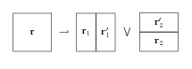
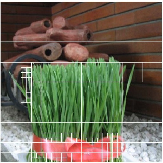
Figure 1: The bi-tree decomposition method.

Here, we use a novel tree decomposition method called bi-tree [26]. In bi-tree, if the block r is not homogeneous enough, rather than the deterministic choice of the sub-blocks in quad-tree, r is divided either horizontally or vertically (see Figure 1). This is accomplished in the way that the total non-homogeneity of the output gets the least possible. Extensive empirical comparison of bi-tree with quad-tree, given in [26], shows that bi-tree produces fewer blocks, with a more uniform distribution of block sizes. On the contrary, quad-tree splits the image more and produces a more scattered pattern of block sizes. The total homogeneity of the resulting blocks are almost the same in both methods. The achievements of bi-tree have the cost of demanding about four times more computational resources than the quad-tree. As the proposed method works better when blocks have similar sizes, we use bi-tree in this paper.

3.3 Basis Vector Polarization

There is a manipulated form of the well-known Euler angles that relates any right-rotating orthonormal matrix with three angles, in a one-to-one revertible transformation [42]. As such, for the matrix V, with its i-th column denoted as [(v)\vec]_i, we write V ~ (q,f,y) when,

ì
ï
í
ï
î

q = Ð([(v)\vec]₁^xy,[1,0]^T)

f = Ð((R_q^xy[(v)\vec]₁)^xz,[1,0]^T)

y = Ð((R_f^xzR_q^xy[(v)\vec]₂)^yz,[1,0]^T)

(5)

Here, Ð([(v)\vec],[(u)\vec]) is the angle between the two vectors [(v)\vec],[(u)\vec] Î R² and [(v)\vec]_p denotes the project of the vector v on the plane p. Also, R_a^p is the 3×3 matrix of a radians counter-clock-wise rotation in the p plane:

ì
ï
ï
ï
ï
ï
ï
ï
ï
í
ï
ï
ï
ï
ï
ï
ï
ï
î

R_q^xy=

é
ê
ê
ê
ë

cosq

-sinq

sinq

cosq

ù
ú
ú
ú
û

R_f^xz=

é
ê
ê
ê
ë

cosf

-sinf

sinf

cosf

ù
ú
ú
ú
û

R_y^yz=

é
ê
ê
ê
ë

cosy

-siny

siny

cosy

ù
ú
ú
ú
û

(6)

It can be proved that to produce V out of the triple (q,f,y) one may use [43],

V=R_-q^xyR_-f^xzR_-y^yz.

(7)

Note that (R^p_a)^-1=R^p_-a. While equation (5) computes the three angles q, f and y out of V, equation (7) reconstructs V from q, f and y. These methods are called polarization and depolarization of a right-rotating orthonormal matrix, respectively [42].

3.4 Block-Wise Interpolation

Consider a partition of the H×W square as a set of rectangular regions {r_i|i=1,¼, n}, while the values of {l_i|i=1,¼, n} are given, satisfying,

) @ l_i, "i, "

Î r_i,

(8)

for an unknown function f:\mathbbR²® \mathbbR. The problem is to properly approximate f as [f\tilde]. We address this problem as block-wise interpolation of the set {(r_i;l_i)|i=1,¼, n}.

Note that, for a conventional rectangular grid as the partition, the problem reduces to an ordinary 2-D interpolation task. Here, we use a reformulated version of the well-known low-pass Butterworth filter, as the interpolation kernel, to carry out the interpolation in the more general case.

ì
ï
ï
í
ï
ï
î

B_t,N(x)=(1+ ([ x/(t)] )^2N)^-¹/₂

ì
ï
í
ï
î

N=rnd(log_{^a/_b}([(bÖ{1- a²})/(aÖ{1-b²})]))

t = a^2NÖ{[(a²)/(1-a²)]}

(9)

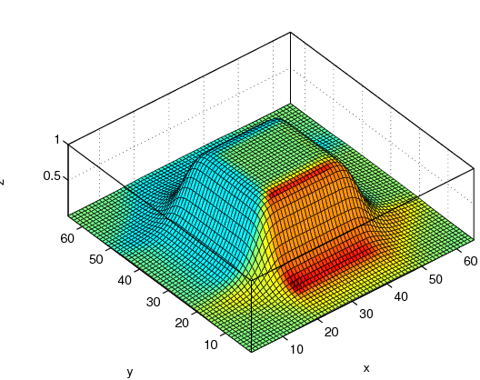
Here, a, b, a and b are given and the function B_t,N(·) satisfies B_t,N(a)=a and B_t,N(b)=b. The 2-D version of this function can be defined as, B_t,N^w,h(x,y)=B_wt,N(x)B_ht,N(y), where w and h control the spread of the function in the x and y directions, respectively. Figure 2 shows the typical shape of the function B_t,N^w,h(x,y) with a=0.9, a = 0.7, b=1, b = 0.5 and w=h=16.

Figure 2: The typical shape of the proposed interpolation kernel, B_t,N^w,h(x,y).

Assuming that the region r_i is centered at (x_i,y_i), while its height and width are w_i and h_i, respectively, we propose the function [f\tilde] to be defined as,

(x,y)=

N
å
i=1

l_iB_t,N^{[(w_i)/2],[(h_i)/2]}(x-x_i,y-y_i)

N
å
i=1

B_t,N^{[(w_i)/2],[(h_i)/2]}(x-x_i,y-y_i)

(10)

Note that, [f\tilde] is a smooth version of the staircase function f.

As the generalization of the block-wise interpolation problem, assume that the set of regions and the corresponding l_ijs are given as {(r_i;l_i1,¼,l_im)|i=1,¼, n}, satisfying, f_j([(c)\vec]) @ l_ij, "i, j, [(c)\vec] Î r_i, for a set of m unknown functions f_j:\mathbbR²® \mathbbR. To solve this problem, in a way similar to (10), we calculate,

(x,y)=

n
å
i=1

l_ijB_t,N^{[(w_i)/2],[(h_i)/2]}(x-x_i,y-y_i)

n
å
i=1

B_t,N^{[(w_i)/2],[(h_i)/2]}(x-x_i,y-y_i)

(11)

Here, because the set of base regions for all [f\tilde]_js are the same, the total performance is increased by computing the kernel just once, for each value of i. Then, the problem reduces to m times computation of a weighted average.

When working in the polar coordinates, ordinary algebraic operations on the variables lead to spurious results, because of the 2p discontinuity. To overcome this problem, rather than directly solving {(r_i;q_i)|i=1,¼, n}, we solve the problem {(r_i;cosq_i,sinq_i)|i=1,¼, n} and then find q_i using ordinary trigonometric methods.

3.5 Eigenimage Theory

Consider the PCA matrix, V_r and the expectation vector, [(h)\vec]_r, corresponding to the homogeneous set r. For the arbitrary color vector [(c)\vec], which belongs to r, the PCA coordinates are calculated as, [(c)\vec]¢=V_r^-1([(c)\vec]-[(h)\vec]_r) [44]. Assume that there exists a method for finding an appropriate color set r_[(c)\vec] for each color vector [(c)\vec]. Here, r_[(c)\vec] describes the color content of [(c)\vec], in the sense that,

=V_{r_[(c)\vec]}^-1

æ
è

r_[(c)\vec]

ö
ø

(12)

satisfies,

s_c¢₁ >> s_c¢₂ >> s_c¢₃,

(13)

where, [(c)\vec]¢=[c¢₁,c¢₂,c¢₃]^T. We call the c¢₁, c¢₂ and c¢₃ components as the pc₁, pc₂ and pc₃, principal components, respectively. The original image can be perfectly reconstructed using these three components, except for numerical errors, as,

=V_{r_[(c)\vec]}

r_[(c)\vec]

(14)

It is proved in [6], theoretically, and in [40], empirically, that for homogeneous swatches, neglecting pc₃ (or even both pc₂ and pc₃), gives good approximation of the original image. These are called partial reconstructions. Note that the perfect reconstruction scheme of (14) does not rely on (13), while the properness of the partial reconstructions defined as,

=V_{r_[(c)\vec]}

é
ê
ê
ê
ë

c¢₁

c¢₂

ù
ú
ú
ú
û

r_[(c)\vec]

(15)

and,

=V_{r_[(c)\vec]}

é
ê
ê
ê
ë

c¢₁

ù
ú
ú
ú
û

r_[(c)\vec]

(16)

do rely on (13).

Now, the goal is to devise an efficient method for calculating, and storing, V_{r_[(c)\vec]} and [(h)\vec]_{r_[(c)\vec]} for all the pixels in an image. In the following, a method for doing this task is proposed.

After feeding an image I into the bi-tree method, The output is the matrix U which contains the coordinates of r_i along with the expectation matrix [(h)\vec]_i and the polarized version of the PCA matrix (q_i,f_i,y_i). Now, consider solving the problem {(r_i;x_i)|i=1,¼, n} using the block-wise interpolation, where x_i is the row vector containing h_i1, h_i2, h_i3, q_i, f_i and y_i. The solution will be the functions [(h)\tilde]₁, [(h)\tilde]₂, [(h)\tilde]₃, [(q)\tilde], [(f)\tilde], [(y)\tilde]: \mathbbR²®\mathbbR. Now, we compute the functions [([(h)\vec])\tilde]:\mathbbR²® \mathbbR³ (expectation map, Emap) and [(V)\tilde]:\mathbbR²® \mathbbR⁹ (rotation map, Rmap), as the expectation vector and the PCA matrix in each pixel, respectively. This leads to the computation of the three eigenimages pc₁, pc₂ and pc₃ (using (12)).

It can be shown that [45],

s_pc₁²+s_pc₂²+s_pc₃²=s_r²+s_g²+s_b²,

(17)

Here, r, g and b are the original RGB components of I. Thus, we define,

k_i=

s_pc₁²

s_pc₁²+s_pc₂²+s_pc₃²

(18)

as the energy ratio of the i-th eigenimage. Now, if the PCA matrix is chosen properly,

k₁ >> k₂ >> k₃.

(19)

In the next two sections, we will show how the eigenimage can be used for effective compression and watermarking of color images.

3.6 Color Image Compression

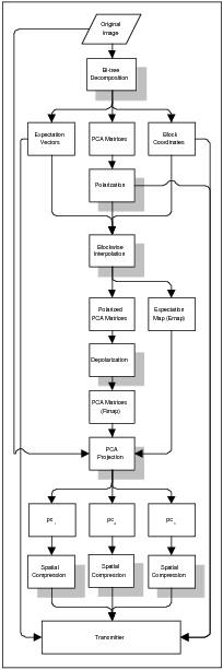
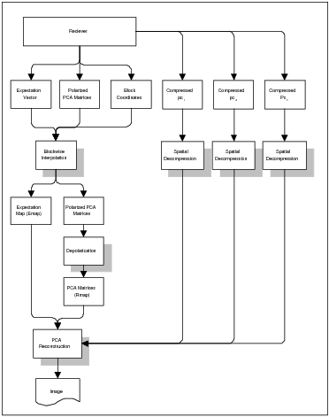
Consider the image I and its corresponding eigenimages pc₁, pc₂ and pc₃. Due to the energy compaction condition, given in (19), this scheme can lead to a spectral compression of an image. As such, reconstructing the image using just one or two eigenimage(s) gives the compression ratios of ³/₂:1 and 3:1, respectively. To add spatial compression to the this scheme, we use the PU-PLVQ gray-scale image compression technique [46] for each eigenimage, independently, with different compression ratios. This leads to the color image compression method proposed in Figure 3.


(a)	(b)

Figure 3: Flowchart of the proposed color image compression method. (a) Compression. (b) Decompression.

As Figure 3-a shows, the transmitted information consists of the compressed versions of pc₁, pc₂ and pc₃, along with U, a, a, b and b. Assume that the compression is to be applied on an H×W image, decomposed into n blocks by the bi-tree method. The total amount of information to be sent equals 10n bytes for storing x_i1, x_i2, y_i1, y_i2, h_i1, h_i2, h_i3, q_i, f_i and y_i plus WH(l₁^-1+l₂^-1+l₃^-1) bytes for storing pc₁, pc₂ and pc₃ eigenimages compressed with compression ratios of l₁, l₂ and l₃, respectively (where l₁ > l₂ > l₃). Thus, the total compression ratio equals,

l @

l₁^-1+l₂^-1+l₃^-1+

10n

(20)

Picking the values of l₂=l₁ and l₃=¥ leads to l @ 1.5l₁. Note that using a pure spatial compression approach, all three color components must be compressed with almost the same compression ratios, resulting in a total compression ratio of l₁. Thus, in the worst case, the proposed method multiples the compression ratio by at least 1.5.

As shown in Figure 3-b, in the decompression process, first, the Emap and the Rmap are computed. Using this information, along with the decoded versions of pc₁, pc₂ and pc₃, the original image is then reconstructed.

3.7 Color Image Watermarking

Consider the image I with the three corresponding eigenimages of pc₁, pc₂ and pc₃. Although, there is no orthogonality constraint in the eigenimage theory, the eigenimage approach can be adapted for watermarking purposes. Assume that the gray-scale watermark image W is to be embedded into I. Also, assume that I and W are of the same size (H×W). First, the dynamic range of W is fitted into that of pc₃, as,

s_pc₃

s_W

(W-h_W).

(21)

Now, replacing pc₃ with the scaled version of the watermark signal, [(W)\tilde], the watermarked image, I¢, is constructed.

The process of extracting the watermark is through computation of the eigenimages corresponding to I¢, which we call pc₁¢, pc₂¢ and pc₃¢. Now, pc₃¢, when normalized, contains the reconstructed watermark signal,

W¢=255

pc₃¢-(h_pc₃¢-s_pc₃¢)

2s_pc₃¢

(22)

4 Experimental Results

The proposed algorithms are developed in MATLAB 6.5, on an 1100 MHz Pentium III personal computer with 256MB of RAM. For a typical 512×512 image it takes 8.3 seconds to extract the eigenimages. Then, another 4.6 seconds are needed to reconstruct the image. Adding the less than one second needed to do the spatial compression, the total operation takes slightly less than 16 seconds for a typical image. It takes a similar amount of time to embed a watermark in a 512×512 image and about 9 seconds to extract it. Note that these values are measured using MATLAB code and can be reduced drastically if the code is implemented using a higher-level programming language.

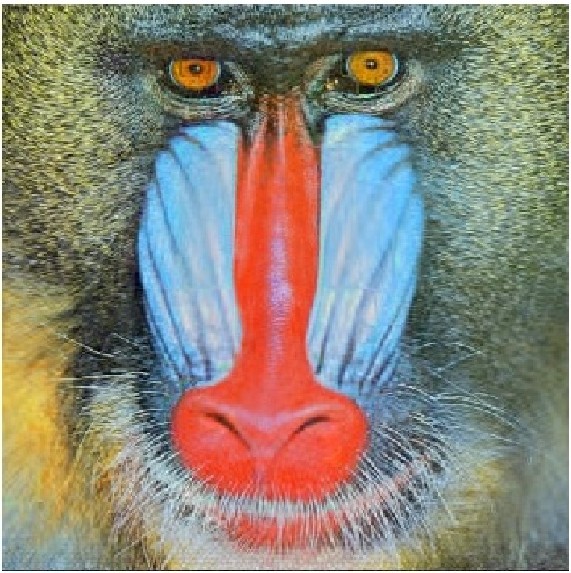
A database of color images which includes the standard images of Lena, Mandrill, Peppers and Couple as well as some professional color photographs [47], a total of 140 images, is used in this research. All images are of the size 512×512, in RGB color space, and are compressed using standard JPEG with qualities above 95. Prior to the operation, all the images are converted to the standard BMP format.

4.1 Block-Wise Interpolation


(a)	(b)

Figure 4: Proposed block-wise interpolation. (a) Sample problem. (b) The solution provided by the proposed block-wise interpolation (SNR > 22dB).

To illustrate the results of the proposed block-wise Interpolation method, a sample problem is given in Figure 4-a, with the associated outcome in Figure 4-b, at the Signal to Noise Ratio (SNR) of more than 22dB.

4.2 Eigenimages

(a)


(b)	(c)	(d)

(e)	(f)	(g)

(h)


(i)	(j)	(k)

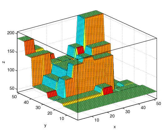
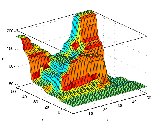
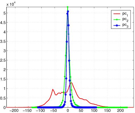
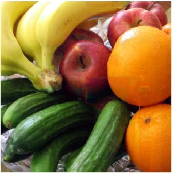
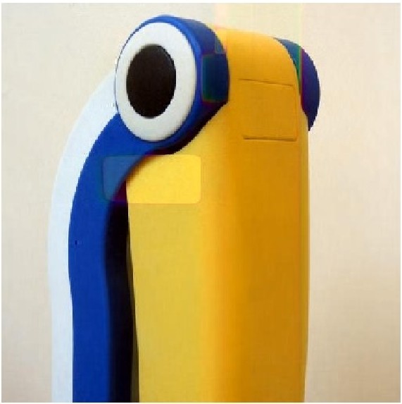
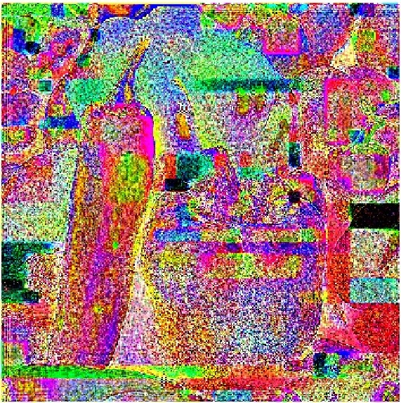
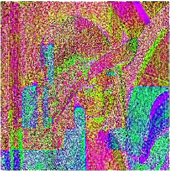
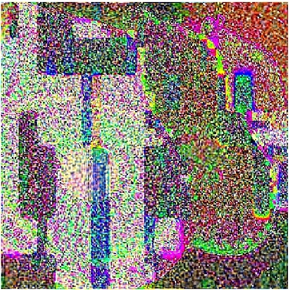
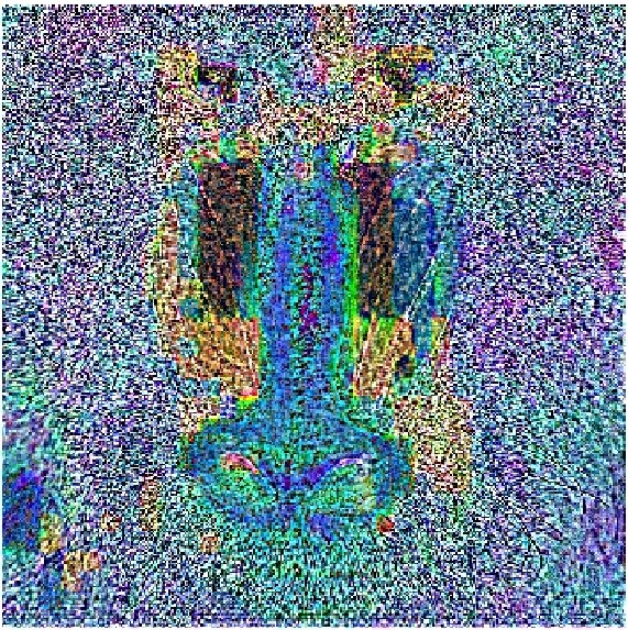
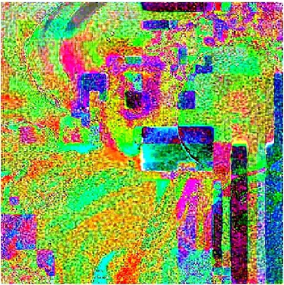
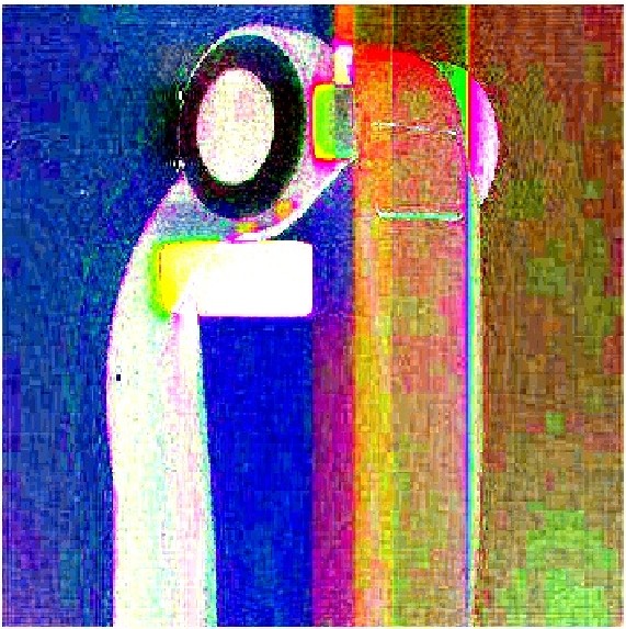
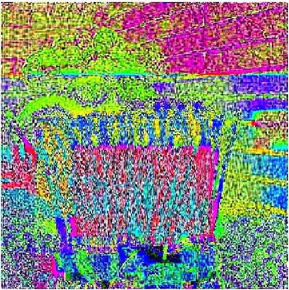
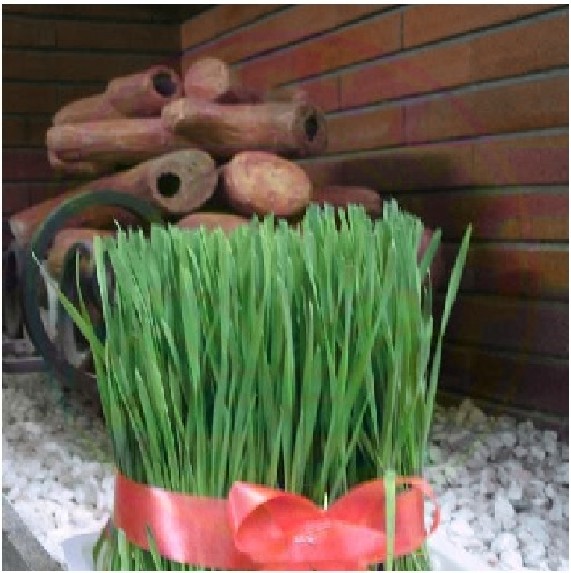
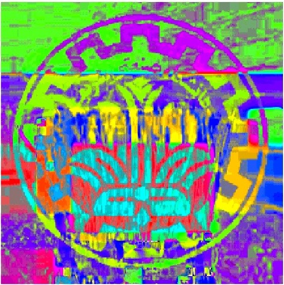
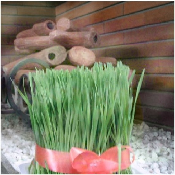
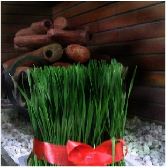
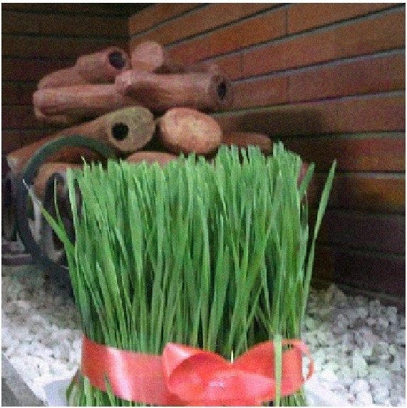
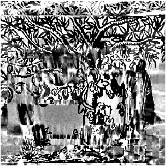
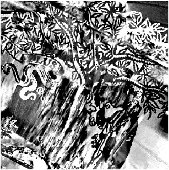
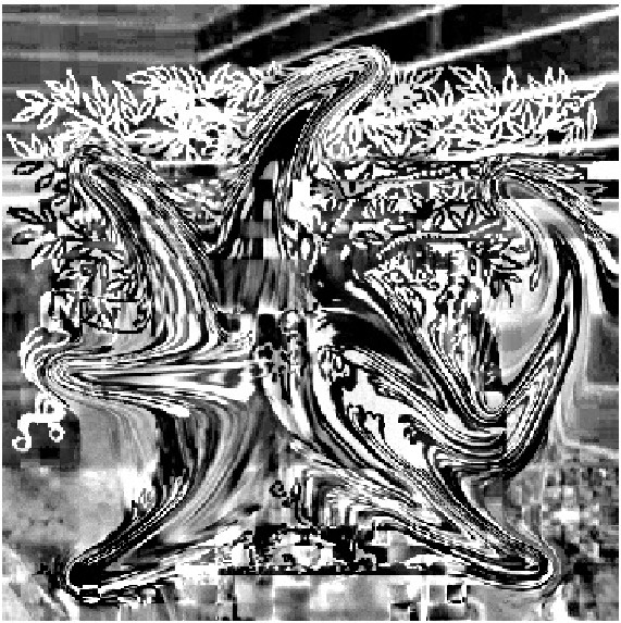
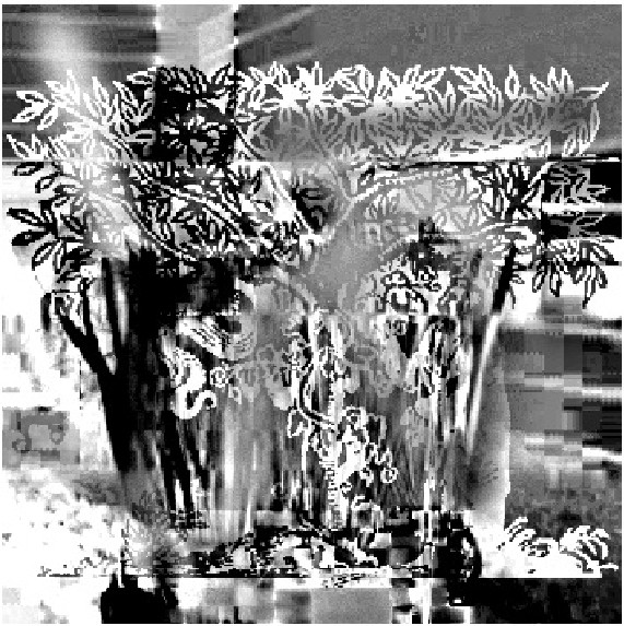
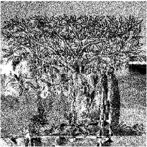
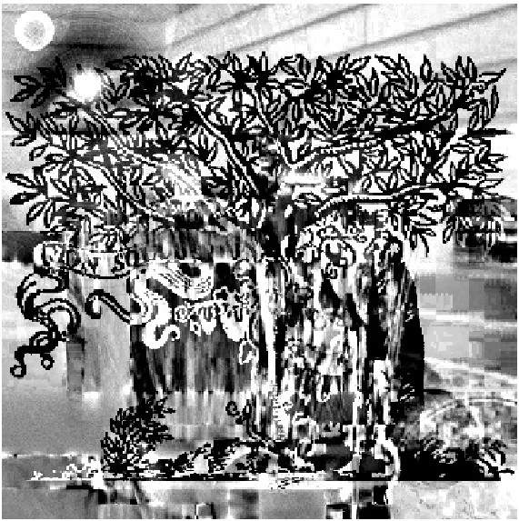
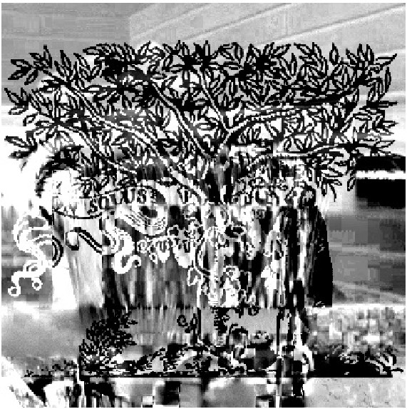
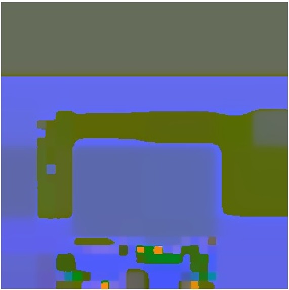
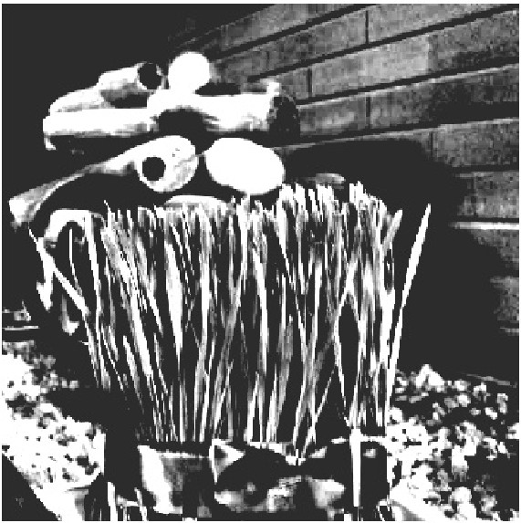
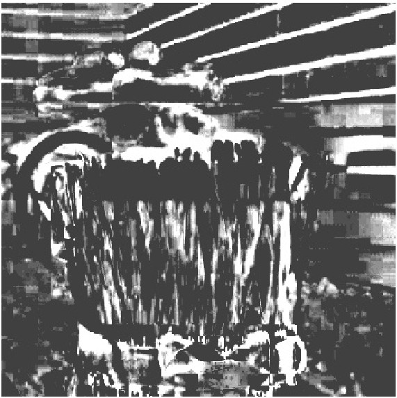
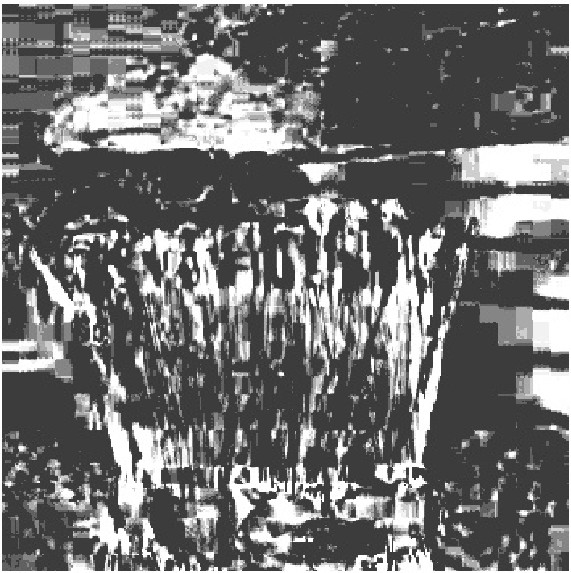
Figure 5: The process of extracting the eigenimages from an arbitrary image. (a) Original image adopted from [47]. (b) Outcome of the bi-tree decomposition method. (c) Emap. (d) Rmap. (e) pc₁. (f) pc₂. (g) pc₃. (h) Histograms of the eigenimages. (i) Reconstruction using all eigenimages (PSNR=60dB). (j) Ignoring one eigenimage (PSNR=38dB). (k) Ignoring two eigenimages (PSNR=31dB).

Figure 5 shows the process of extracting the eigenimages corresponding to the image shown in Figure 5-a, using the proposed method. First, using the bi-tree method with the parameters e₁=5 and r = 5, the image is split into 91 blocks (see Figure 5-b). These blocks are then used to generate the EMap and the RMap, as shown in Figures 5-c and (d), respectively. Subsequently, the eigenimages, as shown in Figures 5-e, f and g, are extracted. Notice that the dynamic ranges of all eigenimages are exaggerated to give a better visualization. The stochastic distributions of the eigenimages are investigated in Figure 5-h. These histograms show the compaction of the energy as discussed next. Using numerical measures, the standard deviations of the eigenimages are computed as, s_pc₁=52, s_pc₂=12 and s_pc₃=6. This results in k₁=94%, k₂=5%, and k₃=1%, a clear compaction of the energy in the first eigenimage.

Figure 5-i shows the result of reconstructing the image shown in Figure 5-a using all three eigenimages. Similarly, Figures 5-j and k show the results of ignoring pc₃ and both pc₃ and pc₂, respectively. The resulting PSNR values are 60dB, 38dB and 31dB, respectively. Note that PSNR of 60dB (instead of infinity), for reconstructing the image using all eigenimages, is caused by numerical errors, while the two other PSNR values (38dB, 31dB) show some loss of information. In the literature, PSNR values of above 38dB are considered visually satisfactory even for professionals [48].

(a)

(b)

(c)

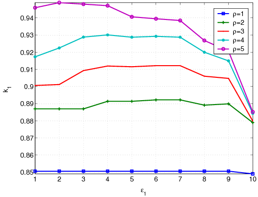
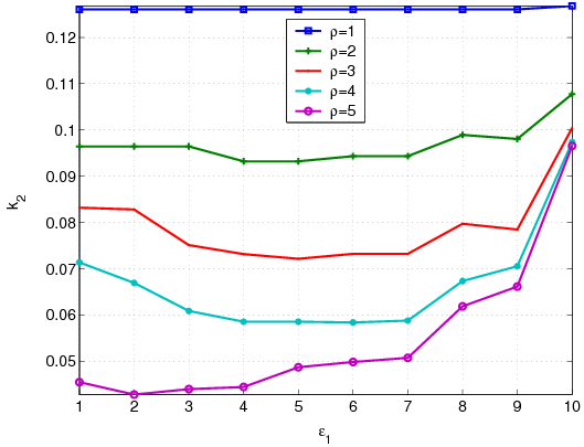
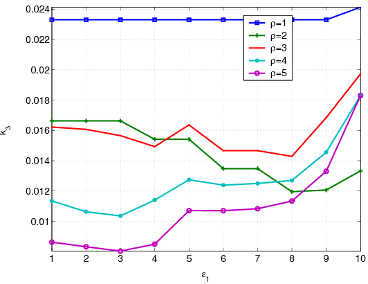
Figure 6: Distribution of energy between the three eigenimages, for different values of e₁ and r. (a)k₁. (b)k₂. (c)k₃.

Figures 6-a, b and c show the values of k₁, k₂ and k₃ for the image shown in Figure 5-a, at different values of e₁ and r. Note that, except for the trivial cases of r £ 2 and e₁ > 9, which are never used in practice, more than 90% of the image energy is stored in pc₁, while pc₂ and pc₃ hold about 9% and 1% of the energy, respectively. Having in mind that in the original image k_r=38%, k_g=32% and k_b=30%, the energy compaction of the eigenimages are considerable.

(a)

(b)

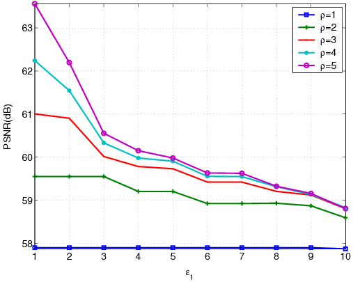
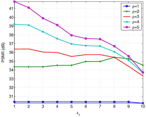
(c)

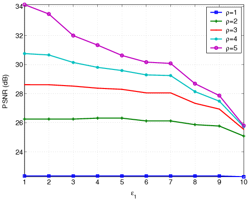
Figure 7: PSNR values corresponding to partially-reconstructed images, for different values of e₁ and r. (a) Using three eigenimages. (b) Using two eigenimages. (c) Using only one eigenimage.

Figure 7 shows the PSNR values obtained by reconstructing the image shown in Figure 5-a using all three eigenimages (Figure 7-a), two eigenimages (Figure 7-b), and only one eigenimage (Figure 7-c), for different values of e₁ and r. Note that, for values of e₁ £ 8 and r ³ 3, reconstructing the image using all eigenimages gives the high PSNR value of about 60dB, while neglecting one and two eigenimages results in PSNR ³ 35dB and PSNR ³ 28dB, respectively.

4.3 Color Image Compression


(a)	(b)	(c)	(d)

(e)	(f)	(g)

Figure 8: Results of the proposed compression method. For details about compression ratio and PSNR see Table 1.


(a)	(b)	(c)	(d)

(e)	(f)	(g)

Figure 9: Exaggerated error of the proposed compression method.

Table 1: Numerical information corresponding to the results shown in Figure 8. [n: block count. l: Compression Ratio, bpp: bit per pixel.]

Sample	Proposed Method										JPEG	JPEG2000
	n	pc₁		pc₂		pc₃		Total
		l	bpp	l	bpp	l	bpp	l	bpp	PSNR (dB)	PSNR (dB)	PSNR (dB)

8-a	334	42.6:1	0.19	58.8:1	0.14	¥	0	71.1:1	0.34	28.4	26.8	27.1
8-b	60	43.1:1	0.19	56.2:1	0.14	¥	0	72.6:1	0.33	33.6	28.9	30.7
8-c	161	39.8:1	0.20	55.1:1	0.15	¥	0	68.0:1	0.35	30.4	27.7	29.5
8-d	311	44.4:1	0.18	58.0:1	0.14	¥	0	72.5:1	0.33	24.5	19.8	21.7
8-e	203	41.3:1	0.19	56.9:1	0.14	¥	0	70.1:1	0.34	33.3	30.5	32.4
8-f	32	45.5:1	0.18	62.8:1	0.13	¥	0	78.8:1	0.30	26.1	38.4	42.4
8-g	91	41.3:1	0.19	57.7:1	0.14	¥	0	71.4:1	0.34	35.4	30.2	32.7

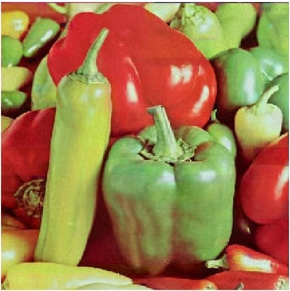
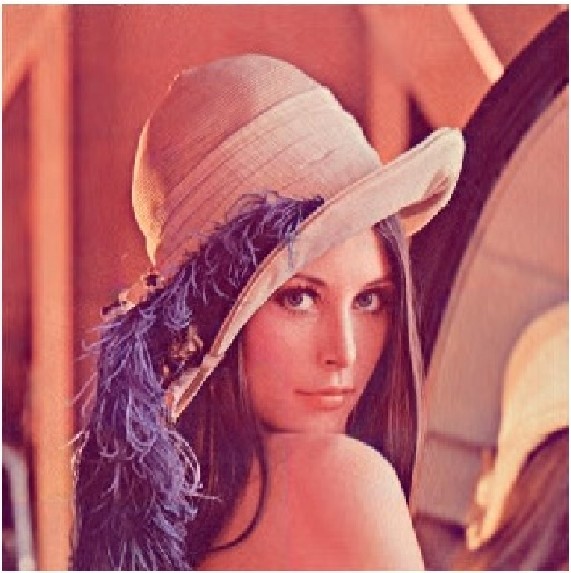
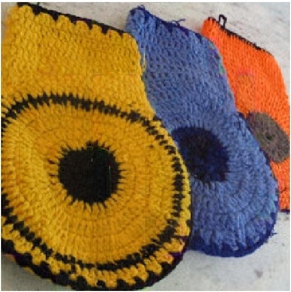
Figure 8 shows the results of the proposed compression method, with the associated numerical values mentioned in Table 1. These results are acquired using e₁=5 and r = 5. To compare the compressed images with the original ones, the exaggerated differences are carried in Figure 9. Note the high compression ratio of about 70:1 in all cases, while the PSNR is mostly above 25dB.

Among other region-based coding approaches, the method by Carveic et. al. is one of the best [9]. In that work, the authors mixed the color and texture information into a single vector and then performed the coding using a massively computationally-expensive algorithm. However, the final results show PSNR values of about 40dB for compression ratios of about 20:1. In [33], the researchers separate the compression in the two disjoint domains of spectral and spatial redundancy, by using a PCA neural network. They reach the compression ratio of 3.7:1 with PSNR of around 25dB, while almost all test samples are homogeneous. In [49], the method gives the compression ratio of about 14.5:1 but with the same range of PSNR as ours. As a more recent approach, we compare the PSNR of 31.93dB reported in [19] for Lena at 1.17bpp with the results of the proposed method in which PSNR of 33.6dB is achieved at 0.33bpp.

Table 1 also compares the proposed algorithm with JPEG and JPEG2000. To do this comparison, each sample image is compressed using each one of these algorithms with the exact compression ratio acquired from the proposed method. As expected, Table 1 shows that JPEG2000 is always giving a better result compared to JPEG. Comparing the proposed method with JPEG2000, we understand that, except for the case of Figure 8-f, the proposed method is giving a higher PSNR than both others. Numerically, the proposed method is 14% and 7% better than JPEG and JPEG2000, respectively, in terms of PSNR. This means more than 3.6dB and 1.9dB increase in the quality when comparing the results of the proposed method with JPEG and JPEG2000, respectively.

4.4 Color Image Watermarking


(a)	(b)

(c)	(d)

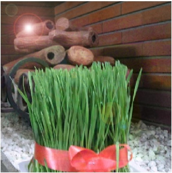
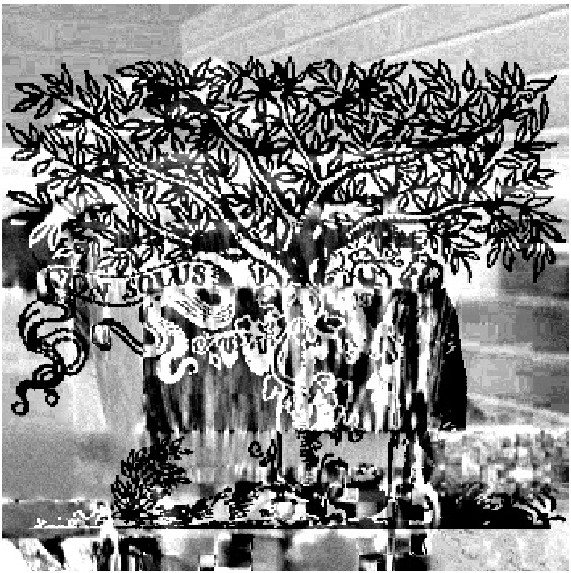
Figure 10: Results of the proposed watermarking method performed on the image shown in Figure 5-a. (a) Watermark data. (b) Watermarked image at PSNR=35dB. (c) Exaggerated difference between the original image and the watermarked image. (d) Extracted watermark data.

To demonstrate the utilization of the proposed method in embeding a watermark in an image, we use the example shown in Figure 10. Here, Figure 10-b shows the results of embedding the watermark data shown in Figure 10-a into the image shown in Figure 5-a. The resulting PSNR of this operation is 35dB. Figure 10-c shows the exaggerated difference between the original image and the watermarked image, and Figure 10-d shows the extracted watermark. Investigating Figure 10-c shows where the proposed method hides the data; at each pixel, the direction of the third principal component shows the direction in which data can be put such that it does not affect the visual perception of the image.

Figure 11: Sample watermark.


(a)	(b)	(c)	(d)

(e)	(f)	(g)	(h)

(i)	(j)	(k)	(l)

Figure 12: Some attacked watermarked images, corresponding items in Table 2 are: (a):1, (b):2, (c):3, (d):5, (e):9, (f):11, (g):12, (h):13, (i):14, (j):23, (k):28, and (l):29


(a)	(b)	(c)	(d)

(e)	(f)	(g)	(h)

(i)	(j)	(k)	(l)

Figure 13: Extracted watermarks from attacked images shown in Figure 12.

Table 2: Some of the attacks performed on the watermarked images to analyze the robustness of the proposed watermarking method.

index	Attack

0	-
1	Enhancement
2	Scaling and trimming
3	Rotation, scaling and trimming
4-7	Nonlinear Geomtrical
8	Gaussian Lowpass
9,10	Scratch
11,12	Local brightening/darkening
13	Text
14	Motion Blur
15	Radial Blur
16-22	Geometrical Distortion
23	Uniform Color Noise
24	Gaussian Color Noise
25	Uniform Gray Noise
26	Gaussian Gray Noise
27	Median
28	Artistic Lens Flare
29	Lossy Compression

To test the robustness of the proposed watermarking method against invasive attacks, the watermark shown in Figure 11 is embedded in the sample image shown in Figure 5-a. Then, the watermarked image is attacked, using Adobe Photoshop 6.0, as stated in Table 2. Figure 12 shows some of the attacked watermarked images and Figure 13 show the corresponding extracted watermark data. Investigating Figure 13 shows that the proposed watermarking method is robust against linear and nonlinear geometrical transformations, including rotation, scaling, trimming, and other geometrical distortions. Also, it is robust against occlusion, artistic effects, noise, enhancement operations such as brightening and increasing contrast (even when performed locally), and also lossy compression for ratios up to 15:1.

Table 3: Comparison of different watermarking approaches with the proposed method, all used in a 512×512 image. -: Not Resistant. ~ : Partially Resistant. Ö: Completely Resistant. [Abbreviations: G: Grayscale, SCC: Single Color Component, CV: Color Vector, LG: Linear Geometrical Transformation, NLG: Nonlinear Geometrical Transformation, LPO: Linear Point Operations, NLPO:Nonlinear Point Operations, SO: Spatial Domain Operations, EO: Editing Operations, CMP: JPEG Compression].

Method

[50]

[51]

[52]

[38]

[36]

[53]

[54]

[55]

[56]

[57]

[58]

Proposed

Capacity

4KB

8KB

2KB

1KB

16KB

0.5KB

60B

64B

2KB

64KB

Domain

SCC

NLG

LPO

NLPO

CMP

Table 3 compares the proposed watermarking method with some of the approaches available in the literature. The table lists the watermark capacity of each method when embedding to a 512×512 color image along with the domain in which the data is embedded. Also, the attack resistance of different approaches is compared here.

It is observed in different experiments that the standard deviation of pc₃ in a typical image is more than 4. Thus, using the proposed watermarking method on a 512×512 color image, at least a same-sized 2bpp image can be used as the watermark signal. This makes the watermark capacity of the proposed method equal to 64KB. This is four times more than the highest capacity of the best available approach [53]. It is worth to mention that only the approaches discussed in [38,58] use color vectors and that only [38] exhibits levels of resistance to linear point operations such as brightening and contrast enhancement. It must be emphasized that that method's resistance is limited to global operations, while the method proposed in this paper is resistant even to local linear point operations (see Figures 12-f and g). Unfortunately, in the literature, minor attention is paid to non-linear geometrical operations, such as elastic and perspective transformation, and image editing processes, such as adding text, artistic effects, occlusion and so on, whilst the copyrighted images can be used in books, posters and websites where they appear in manipulated forms.

5 Conclusion

In this paper, a PCA-based distance function and the corresponding homogeneity criterion are utilized within a tree decomposition method. The resulting decomposition is then used in order to extract the eigenimages associated with a given image. The proposed eigenimage extraction method is proved to be highly efficient in compacting the image energy as well as in providing proper partial reconstructions of color images. The eigenimages are then used in a color image compression method. Furthermore, the fact that manipulating the third eigenimage has minor effect on the quality of an image is used in a novel watermarking method. Both methods are compared with the available literature. Comparison shows that the proposed compression method is superior to the available approaches (in average 1.9dB more than JPEG2000 in PSNR for the samples used in this paper). The analysis of the proposed watermarking method shows that it is resistant to local alterations as well as to the manipulations performed in publications and websites, such as adding text and non-linear geometrical distortions. No other watermarking approach in the literature is found to claim similar resistance.

Acknowledgement

We wish to thank the respected referees for their constructive suggestions. The first author wishes to thank Ms. Azadeh Yadollahi for her encouragement and invaluable ideas. We also thank the photographers Ms. Shohreh Tabatabaii Seifi and Mr. Ali Qanavati for allowing us to use their rich digital image archive.

References

[1]: N. Papamarkos, C. Strouthopoulos, I. Andreadis, Multithresholding of color and gray-level images through a neural network technique, Image and Vision Computing 18 (2000) 213-222.
[2]: D. Tschumperle, PDE based regularization of multivalued images and applications, Ph.D. thesis, University of Nice, Sophia Antipolis (2002).
[3]: H. Cheng, J. Li, Fuzzy homogeneity and scale-space approach to color image segmentation, Pattern Recognition 36 (2003) 1545-1562.
[4]: T. Chaira, A. Ray, Fuzzy approach for color region extraction, Pattern Recognition 24 (2003) 1943-1950.
[5]: L. Lucchese, S. Mitra, Colour segmentation based on separate anisotropic diffusion of chromatic and achromatic channels, Vision, Image, and Signal Processing 148(3) (2001) 141-150.
[6]: G. J. Klinker, S. A. Shafer, T. Kanade, The measurement of highlights in color images, International Journal of Computer Vision 2 (1988) 7-32.
[7]: S.-C. Cheng, S.-C. Hsia, Fast algorithms for color image processing by principal component analysis, Journal of Visual Communication and Image Representation 14 (2003) 184-203.
[8]: J. Limb, C. Rubinstein, Statistical dependence between components of a differentially quantized color signal, IEEE Transactions on Communications 20 (1971) 890-899.
[9]: D. Carevic, T. Caelli, Region-based coding of color images using karhunen-loeve transform, Graphical Models and Image Processing 59(1) (1997) 27-38.
[10]: F. Masulli, A. Massone, A. Schenone, Fuzzy clustering methods for the segmentation of multimodal medical volumes (invited), in: P. Szczepaniak, P. Lisboa, S. Tsumoto (Eds.), Fuzzy Systems in Medicine. Series Studies in Fuzziness and Soft Computing, editor J. Kacprzyk, Springer-Verlag, Heidelberg (Germany), 2000, pp. 335-350.
[11]: L. Lucchese, S. Mitra, Color image segmentation: A state-of-the-art survey (invited paper), Image Processing, Vision, and Pattern Recognition, Proc. of the Indian National Science Academy (INSA-A) 67, A, No. 2 (2001) pp. 207-221.
[12]: T. Q. Chen, Y. Lu, Color image segmentation - an innovative approach, Pattern Recognition 35 (2002) 395-405.
[13]: X. Dai, I. Maeda, Fuzzy-based segmentation of color natural images, in: IEEE ICSP'02, 2002, pp. 969-972.
[14]: S.-H. Leung, S.-L. Wang, W.-H. Lau, Lip image segmentation using fuzzy clustering incorporating an elliptic shape function, IEEE Transaction on Image Processing 13(1) (2004) 51-62.
[15]: K.-K. Ma, J. Wang, Color distance histogram: A novel descriptor for color image segmentation, in: Seventh International Conference on Control, Automation, Robotics, and Vision (ICARCV'02), Singapore, 2002, pp. 1228-1232.
[16]: G. J. Klinker, S. A. Shafer, T. Kanade, A physical approach to color image understanding, International Journal of Computer Vision 4 (1990) 7-38.
[17]: D. O. Nikolaev, P. O. Nikolayev, Linear color segmentation and its implementation, Computer Vision and Image Understanding 94 (2004) 115-139.
[18]: M. Turk, A. Pentland, Eigenfaces for recognition, Journal of Cognitive Neuroscience 3(1) (1991) 71-86.
[19]: B. C. Dharaa, B. Chanda, Color image compression based on block truncation coding using pattern fitting principle, Pattern Recognition 40 (2007) 2408-2417.
[20]: A. Abadpour, Color image processing using principal component analysis, Master's thesis, Sharif University of Technology, Mathematical Sciences Department, Tehran, Iran (June 2005).
[21]: A. Abadpour, S. Kasaei, Performance analysis of three likelihood measures for color image processing, in: IPM Workshop on Computer Vision, Tehran, Iran, 2004.
[22]: Q. Ye, W. Gao, W. Zeng, Color image segmentation using density-based clustering, in: Proceedings of 2003 IEEE International Conference on Acoustic and Signal Processing, Hog Kong, 2003, pp. 401-404.
[23]: H. Samet, Region representation: Quadtrees from boundary codes, Comm. ACM 21 (1980) 163:170.
[24]: C. Faloutsos, H. Jagadish, , Y. Manolopoulos, Analysis of the n-dimensional quadtree decomposition for arbitrary hyperrectangles, IEEE Transaction on Knowledge and Data Engineering 9, No. 3 (1997) 373-383.
[25]: M. Yazdi, A. Zaccarin, Interframe coding using deformable triangles of variable size, in: ICIP'97, 1997, pp. 456-459.
[26]: A. Abadpour, S. Kasaei, A new tree decomposition method for color images, in: 10th Annual CSI Computer Conference (CSICC2005), Tehran, Iran, 2005.
[27]: ITU-R Recommendation BT-601-5: Studio Encoding Parameters of Digital Television for Standard 4:3 and Widescreen 16:9 Aspect Ratios, www.itu.ch/, Geneva, 1994.
[28]: K. Benson, Television Engineering Handbook, Mc Graw-Hill, New York, London, 1992.
[29]: J. Slater, Modern Television System to HDTV and Beyond, Pitman, London, 1991.
[30]: J. O. Limb, C. Rubinstein, J. Thompson, Digital coding of color video signals- a review, IEEE Transaction of Communication 25(11) (1977) 1349-1385.
[31]: W. Pratt, Spatial transform coding of color images, IEEE Transaction on Communication Technology 19(6) (1971) 980-992.
[32]: S. Fukuma, M. Iwahashi, N. Kambayashi, Lossless color coordinate transform for lossless color image coding, 1998, pp. 595-598.
[33]: C. Clausen, H. Wechsler, Color image compression using PCA and back propagation learning, Pattern Recognition 33 (2000) 1555-1560.
[34]: M. Swanson, M. Kobayashi, A. Tewfik, Multimedia data-embedding and watermarking technologies, in: Proceedings of the IEEE, Vol. 86(6), 1998, pp. 1064-1087.
[35]: M. Kutter, F. Jordan, F. Bossen, Digital watermarking of color images using amplitude modulation, Electronic Imaging 7(2) (1998) 326-332.
[36]: P.-T. Yu, H.-H. Tasi, J.-S. Lin, Digital watermarking based on neural networks for color images, Signal Processing 81 (2001) 663-671.
[37]: E. Shahinfard, S. Kasaei, Digital image watermarking using wavelet transform, in: Iranian Conference of Mechatronics Engineering, ICME, Qazvin, Iran, 2003, pp. 363-370.
[38]: C.-H. Chou, T.-L. Wu, Embedding color watermarks in color images, EURASIP Journal on Applied Signal Processing 1 (2001) 327-332.
[39]: C.-S. C. P.S. Huang, C.-P. Chang, T.-M. Tu, Robust spatial watermarking technique for colour images via direct saturation adjustment, IEE Proceedings Vision, Image & Signal Processing 152 (5) (2005) 561-574.
[40]: A. Abadpour, S. Kasaei, A new parametric linear adaptive color space and its PCA-based implementation, in: The 9th Annual CSI Computer Conference, CSICC, Tehran, Iran, 2004, pp. 125-132.
[41]: A. Abadpour, S. Kasaei, A new principle component analysis based colorizing method, in: Proceedings of the 12th Iranian Conference on Electrical Engineering (ICEE2004), Mashhad, Iran, 2004.
[42]: A. Abadpour, S. Kasaei, A new PCA-based robust color image watermarking method, in: The 2nd IEEE Conference on Advancing Technology in the GCC: Challenges, and Solutions, Manama, Bahrain, 2004.
[43]: A. Abadpour, S. Kasaei, Unsupervised, fast and efficient color image copy protection, IEE Proceedings Communications 152 (5) (2005) 605-616.
[44]: H. Hotteling, Analysis of a complex of statistical variables into principal components, Journal of Educational Psychology 24 (1933) 417-441.
[45]: A. Abadpour, S. Kasaei, An efficient PCA-based color transfer, Visual Communication & Image Representation 18 (1) (2007) 15-34.
[46]: S. Kasaei, M. Dericher, B. Biashash, A novel fingerprint image compression technique using wavelet packets and pyramid lattice vector quantization, IEEE Transactions on Image Processing 11(12) (2002) 1365-1378.
[47]: S. T. Seifi, A. Qanavati, Digital color image archive, Qnavati@mehr.sharif.edu.
[48]: S. Katzenbeisser, A. Petitcolas, Information Hiding Techniques for Steganography and Digital Watermarking, Artech House Inc., 2000.
[49]: Y.-D. Yu, D.-S. Kang, D. Kim, Color image compression based on vector quantization using PCA and LEBD, in: IEEE IENCON'99, 1999, pp. 1259-1262.
[50]: J. Ruanaidh, W. Dowling, F. Boland, Watermarking digital images for copyright protection, IEE Proceedings on Vision, Signal and Image Processing 143(4) (1996) 250-256.
[51]: A. Nikoladis, I. Pitas, Robust watermarking of facial images based on salient geometric pattern matching, IEEE Transaction on Multimedia 2(3) (2000) 172-184.
[52]: M.-S. Hsieh, D.-C. Tseng, Y.-H. Huang, Hiding digital watermarks using multiresolution wavelet transform, IEEE Transaction on Industrial Electronics 48(5) (2001) 875-882.
[53]: M. Barni, F. Bartolini, A. Piva, Multichannel watermarking of color images, IEEE Transaction on Circuits and Systems for Video Technology 12(3) (2002) 142-156.
[54]: M. Kutter, S. Winkler, A vision-based masking model for spread-spectrum image watermarking, IEEE Transaction on Image Processing 11(1) (2002) 16-25.
[55]: C.-W. Tang, H.-M. Hang, A feature-based robust digital image watermarking scheme, IEEE Transaction on Signal Processing 51(4) (2003) 950-959.
[56]: X. Kang, J. Huang, Y. Q. Shi, Y. Lin, A dwt-dft composite watermarking scheme robust to both affine transform and jpeg compression, IEEE Transactions on Circuits and Systems for Video Technology 13(8) (2003) 776-786.
[57]: Shih-Hao, Y.-P. Lin, Wavelet tree quantization for copyright protection watermarking, IEEE Transactions on Image Processing 13(2) (2004) 154-165.
[58]: P. Tsai, Y.-C. Hu, C.-C. Chang, A color image watermarking scheme based on color quantization, Signal Processing 84 (2004) 95-106.

File translated from T_EX by T_TH, version 3.72.
On 23 Apr 2008, 12:44.

Color PCA Eigenimages and Their Application to Compression and Watermarking

Arash Abadpour and Shohreh Kasaei

Mathematics Science Department, Sharif University of Technology, Tehran, Iran

Computer Engineering Department, Sharif University of Technology, Tehran, Iran

Abstract

1 Introduction

2 Literature Review

2.1 Distance Functions and PCA-Based Color Image Processing

2.2 Tree Decomposition

2.3 Color Image Compression

2.4 Color Image Watermarking

3 Proposed Method

3.1 Distance Functions and Homogeneity Criteria

3.2 Bi-Tree Decomposition

3.3 Basis Vector Polarization

3.4 Block-Wise Interpolation

3.5 Eigenimage Theory

3.6 Color Image Compression

3.7 Color Image Watermarking

4 Experimental Results

4.1 Block-Wise Interpolation

4.2 Eigenimages

4.3 Color Image Compression

4.4 Color Image Watermarking

5 Conclusion

Acknowledgement

References

Color PCA Eigenimages
and Their Application to Compression and Watermarking