Closed Form Solution for Maximizing the Sum Capacity of Reverse-Link CDMA System with Rate Constraints
Closed Form Solution for Maximizing the Sum Capacity of Reverse-Link CDMA System with Rate Constraints
Arash Abadpour1,2, Attahiru Sule Alfa1,2, and Anthony C.K. Soong3 1 Department of Electrical and Computer Engineering, University of Manitoba, Canada, {abadpour,alfa}@ee.umanitoba.ca 2 TRLabs, Winnipeg, 3 Huawei Technological Co. Ltd., TX, USA, asoong@huawei.com
Abstract
In this paper, we work on maximizing the capacity of the reverse link of a CDMA wireless network. Oh and Soong [1] presented an information-theoretic capacity model for analyzing this system. That formulation produces solutions that often result in unfairness allocation of power to most users. Here, we propose the addition of a maximum capacity constraint into the problem, thereby creating a more fair power allocation scheme. First, we improve on the algorithm presented in [1] by proposing a closed form solution and an algorithm which works nine times faster. Then, we propose a closed form algorithm for solving the new enhanced problem.
Quality of Service, Single Cell, Reverse Link CDMA, Optimization.
With the introduction of multimedia services to wireless CDMA communications, the goal is no more to provide fixed capacity to all users [2], but to maximize the aggregate capacity given a set of constraints [3]. In this paper, we focus on maximizing the capacity of the reverse link (uplink), which is often the limiting link [4]. Note that we are looking at the traffic channels, and not the access channels [5]. We emphasize that power control strategies used in the reverse link are completely different from those utilized in the forward link [6]. This is mainly due to the stringent requirements of the reverse link [7].
Maximizing the capacity of the reverse link in this paper is achieved through controlling the transmission power of the individual stations. The analysis is carried out in a single-cell system by assuming that either there is only one cell in the system or that the activity in other cells can be modeled as interference to the current cell [8]. We also use the term capacity as the rate of transmission of each station. To relate transmission power to rate, we use Shannon's theorem as a maximum bound [3,9]. This approach is adopted from previously developed models (see [10] for example).
The system-wide information theoretic capacity of CDMA systems was first analyzed in [8] and then developed further for multi-user networks [11,3]. While these works focused on the set of all capacities, more recent research has benefited from the advances in matched filters and has analyzed the aggregate capacity [10,12,13]. In these works, assuming a sub-optimal coding scheme, the mapping between signal to interference ratio (SIR) and throughput is determined by the coding strategy. A next development has been the assumption of Shannon capacity. Although, Shannon only gives the maximum bound for the capacity, the existence of coding strategies such as Turbo Coding makes the Shannon bound practically reachable [3].
Here, we first formally define the problem. Assume that there are M mobile stations with reverse link gains of g1,¼, gM, which satisfy g1 > ¼ > gM. Denote the transmit power of the i-th mobile station as pi, 0 £ pi £ pmax where pmax is the maximum transmission power of each station. With a background noise of I, the signal to noise ratio (SNR) for the signal coming from the i-station, as perceived by the base station, is calculated as,
gi=
pigi
I+
M å
j=1,j ¹ i
pjgj
.
(1)
Using C=Blog2(1+g) and omitting the constant B, the aggregate capacity of the system can be written as,
C(
®
p
)=log2
æ è
I+
M å
j=1
pjgj
ö ø
M
M Õ
i=1
æ è
I+
M å
j=1,j ¹ i
pjgj
ö ø
.
(2)
The aim of the optimization problem formulated in [1], which has been improved here, is to find the vector [(p)\vec]=(p1,¼,pM) which maximizes C([(p)\vec]) subject to these constraints,
ì ï ï í
ï ï î
"i, 0 £ pi £ pmax
"i,
pigi
I+åj=1,j ¹ iM pjgj
³ g
M å
i=1
pigi £ Pmax
.
(3)
We call this the classical problem. In [1], the authors showed that the search space of this problem can be reduced from [0,pmax]M to a finite number of one-dimensional spaces. Then, to locate the optimal point, they used a numerical search. This solution was observed to lead to one user receiving a disproportionately higher capacity (power allocation) than the remaining users. This type of result we say is unfair to some users. In addition we find that the algorithm developed in that paper could be improved significantly.
In this paper, we go further and prove that the search space can be reduced to an order of M points, compared to the order of M intervals given in [1]. This way, we eliminate the numerical search stage used in [1] and achieve a higher level of performance and accuracy. We show that using these results the problem is solved much faster. Then, to solve the known unfairness issue about the problem, we add a maximum capacity constraint. Subsequently, we propose a closed form algorithm for solving the new problem and show that the unfairness is limited in the new problem formulation. Finally, we compare the two problems in a time interval, for moving stations.
2 Classical Problem: Improvement to its Solution Technique
In this section we present the summary of our improvements to the classical problem.
Defining the variable xi=pigi/I, the classical problem can be rewritten as minimizing,
F(
®
x
)=
M Õ
i=1
æ è
1+
M å
j=1
xj-xi
ö ø
æ è
1+
M å
j=1
xj
ö ø
M
,
(4)
subject to,
ì ï ï ï í
ï ï ï î
"i, 0 £ xi £ li=
pmax
I
gi
"i,
xi
1+åj=1M xj
³ j =
g
g+1
M å
i=1
xi £ Xmax=
Pmax
I
.
(5)
Because of the special structure of (4) and (5), we focus on the hyperplanes
defined as åi=1Mxi=T for fixed values of T, independently. In such a hyperplane, the problem can be restated as finding the minimum of F([(x)\vec])=(1+T)-MFT([(x)\vec]) where FT([(x)\vec])=Õi=1M(1+T-xi). Then, having fixed T, the problem is to minimize FT([(x)\vec]). Furthermore, in these hyperplanes, the constraints can be written as T £ Xmax and "i, j(1+T) £ xi £ li.
Theorem 1
Consider any i ¹ j, and d, changing xi and xj into xi+d and xj-d, respectively, gives another point on the same hyperplane. In the solution to the classical problem, we establish that |(xi+d)- (xj-d)| £ |xi-xj|.
For proof of this theorem, as well as the proofs for other theorems given in this paper, refer to [14,15]. Then, a modified version of Proposition 1 in [1] is stated as Theorem II,which gives the structure of the optimum solution to the classical problem. Here, the unknowns are k, xk, and T..
Theorem 2If there is any solution to the classical problem, then it is structured as [(x)\vec]=[l1,¼,lk-1,xk,j(1+T),¼,j(1+T)], for a value of k.
The work introduced in [1] stops at this point and uses numerical search for different values of k to find the best xk. Here, we go further and reduce the size of the search space by finding appropriate necessary and sufficient bounds for both k and xk, using Theorem III. This theorem also shows how T is related to k and xk.
Theorem 3 In the optimal solution to the classical problem, we have T=[(xk+L+1)/(1-(M-k)j)]-1, where L=åi=1k-1li. Furthermore, k must satisfy M-[1/(j)]+1 < k < [1/(j)]-[1/(lM)]+1 and xk must comply with mink £ xk £ maxk for,
ì ï ï í
ï ï î
maxk=
min
ì í
î
lk,(Xmax+1)[1-(M-k)j]-L-1,lM
1-(M-k)j
j
-L-1
ü ý
þ
mink=
j(L+1)
1-(M-k+1)j
.
(6)
All these inequalities are both necessary and sufficient.
By reducing the search space from
a set of one-dimensional spaces into a finite set of points we present in Theorem IV how to determine the optimal xk, for a known k. This
is another important contribution of this paper, compared
to [1], where the plausible interval for xk is
numerically searched.
Theorem 4
In the optimal solution to the classical problem, xk must accept one of the marginal values
given in Theorem III.
Using the results produced so far we propose the algorithm Classical Single-Cell (CSC) (for details refer to [14]). This algorithm searches for the optimal solution among less than 2M points, for which closed forms are given. Analysis of the proposed algorithm shows that its computational cost is O(M2) flops, 8M2 flops in the worst case and 2M2 flops in a typical one. The old algorithm needs 75M2 flops. Comparing this with the computational complexity of the proposed algorithm, the proposed one is at least more than nine times faster, usually more than thirt six times faster. It is worth to mention that it can be shown that the actual value of Pmax is important only if Pmax < pmaxgM[(g+1)/(g)]-I.
Experimental analysis shows that in the solution to the CSC problem, every station, except for the first one, is set to transmit at the minimum possible SNR. The first station's transmit power, on the other hand, is only limited by the maximum aggregate power received, or its own maximum power limit. This results in a ratio unfairness of over a thousand, in most cases, where the ratio unfairness, [f\tilde], is defined as the ratio between the maximum and the minimum capacities of the stations.
This was observed in [1,12,13]. In fact, this unfairness was one of the main reasons the authors in [1] included the minimum SNR constraint into the problem. We conjecture that the problem with the solution comes from the fact that the constraints neglect the unfairness of the solution. Furthermore, the formulation ignores the fact that a maximum bound on the capacities of the single stations is also necessary.
Based on the discussion given in Section III, we propose a new constraint to be added to the optimization problem, as "i, Ci £ h. Now, using the definition of xi, and by defining w = 1-2-h, the problem reduces to minimizing FT([(x)\vec]) given T £ Xmax and "i, j(1+T) £ xi £ min{li,w(1+T)}. Note that, because the objective function of this problem is identical to the one for the classical case, Theorem I is still valid. Furthermore, looking at the search space of the new problem, it is a pyramid-like structure. While in the classical problem the maximum bounds were decreasing, in the new problem they are fixed for some initial values of i, where li > w(1+T), and then they start decreasing. Thus, the three lemmas given in [1] are still valid and a theorem similar to Theorem II can be proved similarly for the new problem.
Theorem 5
If there is any solution to the new problem, then it is structured as [(x)\vec]=[w(1+T),¼,w(1+T),lj+1,¼,lk-1,xk,j(1+T),¼,j(1+T)], for a pair of j and k.
Theorem 6
In the optimal solution to the new problem we have T=[1/(y)](xk+L+1)-1 where L=åi=j+1k-1li and y = 1-[jw+(M-k)j]. Furthermore, we must have y > j and minjk £ xk £ maxjk for,
ì ï ï ï ï ï ï í
ï ï ï ï ï ï î
maxjk=
min
ì ï ï ï í
ï ï ï î
lk,
[(w)/(y-w)](L+1),
y > w,
[(y)/(w)]lj -(L+1),
j ¹ 0,
[(y)/(j)]lM - (L+1),
y(Xmax+1)-(L+1),
ü ï ï ï ý
ï ï ï þ
minjk=
max
ì ï í
ï î
[(y)/(w)]lj+1-(L+1),
k > j+1,
[(j)/(y-j)](L+1)
ü ï ý
ï þ
.
(7)
Theorem 7
In the optimal solution to the new problem, xk must accept one of the marginal values given
in Theorem VI.
Using Theorem VII we propose the algorthm New Single Cell (NSC) (for details refer to [15]). This algorithm searches for the optimal solution among less than 2M2 points, for which closed forms are given. Analysis shows that the computational cost of this algorithm is O(M3), 5.3M3 flops in the worst case and 1.3M3 flops in a typical one. We define the subtractive unfairness, f is defined as the difference between these two entities.
It can be shown that in the new problem,
f £ log2
æ è
1-j
1-w
ö ø
@ h-
1
ln2
g,
~
f
£
log2(1-w)
log2(1-j)
@
h
g
ln2.
(8)
Note that such bounds on the unfairness of the system did not exist in the classical problem.
The computer codes for the proposed algorithms are developed in MATLAB 7.0.4 on a PIV 3.00GHZ with 1GB of RAM. The parameters used in this study are g = -50dB, I=-113dBm, and Pmax=-106dBm, pmax=23dBm [16,17] plus h = 0.3. Here, we work on a circular cell of radius R=2.5Km. For the station i at distance di from the base station, we only consider the path loss which is calculated as gi=Cdin [18]. Here, C and n are constants equal to 7.75×10⁻³ and -3.66, respectively, when di is in meters [16].
To compare the results of the two formulations, the same problems are solved in both frameworks. Table I shows the values of gi for a sample example where M is equal to 10. Table I also shows the solutions to the classical and new problems with the set of parameters given in the above. For each problem, first the pattern of the solution is given. Using this pattern we are interested in seeing where the breaking points occur. As also expected from previous research [12,13], the classical solution serves the first station with the maximum possible capacity while the others are left to the minimum guaranteed amount. When we add the maximum capacity constraint, we are in fact limiting the first station's capacity. As seen in the results of the new problem, this results in a more balanced spread of the capacity between more users. Looking at the solution to the new problem, nine users are served at the maximum possible capacity (determined either by h or li) while the tenth one has a value in between.
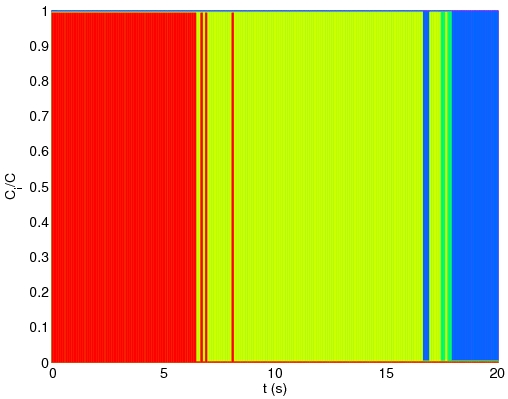
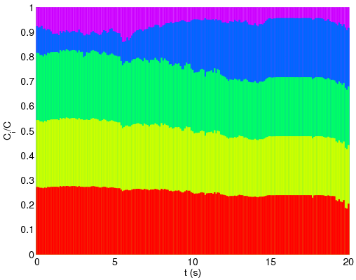
To show this difference more clearly, we define the capacity share of the i-th station as [C\tilde]i=[(Ci)/C]. The capacity shares in both cases are shown in Table I. It is clear that the classical problem produces a solution which is dominantly dependent on the first station, while the solution to the new problem spreads the capacity more evenly among more number of stations.
As expected both from the analysis and from the set of capacity values shown here, the solution to the new problem is more fair than the one produced by the classical problem. In fact, the ratio unfairness measure is about eighty times lower in the new problem compared to the classical one; 6 compared to 518. Note that, here, we see the aggregate capacity becoming smaller in the new problem as a result of adding the maximum capacity constraint.
Here, we carry out another experiment in which M=5 stations move around in a cell as modeled by a discrete random walk with the speed at each moment chosen as a uniform random variable between zero and 5Km/h [19]. Here, we assume that no station leaves or enters the cell. Now, looking at a time span of 20s, the system is solved every 100ms using both algorithms, independently. It is worth to mention that CPU utilization is 7% and 36% for the classical problem and the new one, respectively.
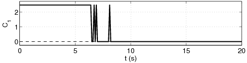
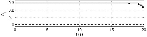
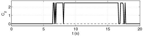
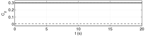
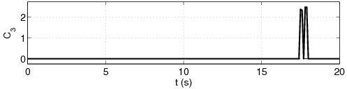
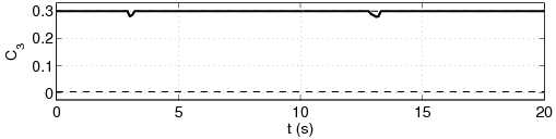
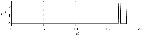
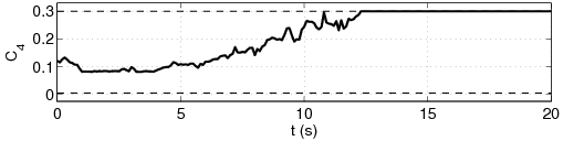
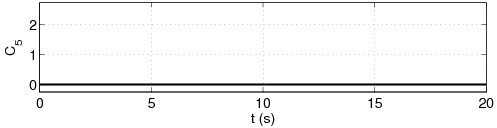
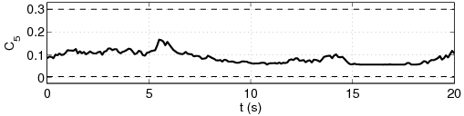
Figure 1 shows the capacity shares of different stations in the two problems over time, where each color indicates one station. As anticipated, the classical problem tends to allocate its entire resources to the closest station at each moment. On the contrary, the new problem only increases its dependency each station as they get closer to the base station. Comparison also shows that the classical problem tends more to force stations to have rapid changes in the power [15]. Furthermore, the capacity curves for the classical problem, given in Figure 2-a, show that the stations are mostly oscillating between two situations of minimum capacity and a very high one. On the other hand, the new problem (see Figure 2-b) keeps the capacity of different cells between the two specified bounds. The significant observation about the solution to the new problem in this example is that the capacity of none of the stations is ever squeezed down to the minimum guaranteed limit (this may not always be true).
In this paper, the problem of optimizing the aggregate system capacity of the reverse link in a single-cell CDMA system was addressed. The formulation was adopted from previous research which also suggested a numerical algorithm for solving the problem. Here, we proposed a closed form algorithm which solves the problem at least nine times faster. Then, to solve the unfairness issue about the problem, we proposed a maximum capacity constraint to be added to it and proposed another closed form algorithm for solving the resulting problem. We also analytically showed that the new constraint gives an upper limit for the unfairness of the solution. This was also presented by solving the two problems for the same set of stations and parameters. Then, we adopted a scenario in which a few stations move around in a cell. We showed that the classical problem tends to limit all stations' capacities to the minimum guaranteed values, while the closest station is granted a very high capacity. The new problem, on the other hand, only increases its dependency on the stations, as they become closer to the base station.
Acknowledgement
The research of A. S. Alfa is partially supported by a grant from NSERC. The first author wishes to thank Ms. Azadeh Yadollahi for her encouragement and valuable discussions. We also appreciate the respected anonymous referees for their constructive suggestions.
S.-J. Oh and A. C. K. Soong, "QoS-constrained information-theoretic sum
capacity of reverse link CDMA systems," IEEE Transactions on
Wireless Communications, vol. 5 (1), pp. 3-7, 2006.
S. Ulukus and L. Greenstein, "Throughput maximization in CDMA uplinks using
adaptive spreading and power control," in IEEE Sixth International
Symposium on Spread Spectrum Techniques and Applications, 2000, pp.
565-569.
A. Viterbi and A. Viterbi, "Erlang capacity of a power controlled CDMA
system," IEEE Journal on Selected Areas in Communications, vol. 11
(6), pp. 892-900, 1993.
D. I. Kim, E. Hossain, and V. K. Bhargava, "Downlink joint rate and power
allocation in cellular multirate WCDMA systems," IEEE Transactions
on Wireless Communications, vol. 2 (1), pp. 69-80, 2003.
S. Verdu, "The capacity region of the symbol-asynchronous gaussian
multiple-access channel," IEEE Transactions on Information Theory,
vol. 35 (4), pp. 733-751, 1989.
R. Knopp and P. Humblet, "Information capacity and power control in
single-cell multiuser communications," in 1995 IEEE International
Conference on Communications, Seattle, 1995, pp. 331-335.
S. Kandukuri and S. Boyd, "Simultaneous rate and power control in multirate
multimedia CDMA systems," in IEEE Sixth International Symposium on
Spread Spectrum Techniques and Applications, NJIT, NJ, 2000, pp. 570-574.
S.-J. Oh, D. Zhang, and K. M. Wasserman, "Optimal resource allocation in
multi-service CDMA networks," IEEE Transactions on Wireless
Communications, vol. 2, pp. 811-821, 2003.
S. A. Jafar and A. Goldsmith, "Adaptive multirate CDMA for uplink throughput
maximization," IEEE Transactions on Wireless Communications, vol. 2,
pp. 218-228, 2003.
A. Abadpour, A. S. Alfa, and A. C. Soong, "QoS-constrained
information-theoretic sum capacity of reverse link cdma systems in a single
cell," Electrical & Computer Engineering Department, University of
Manitoba, Winnipeg, Canada, Tech. Rep., 2006.
--, "Information-theoretic sum capacity of reverse link CDMA systems in
a single cell, a more realistic approach," Electrical & Computer
Engineering Department, University of Manitoba, Winnipeg, Canada, Tech. Rep.,
2006.
T. Rappaport and L. Milstein, "Effects of radio propagation path loss on
DS-CDMA cellular frequency reuse efficiency for the reverse channel,"
IEEE Transactions on Vehicular Technology, vol. 41 (3), pp. 231-242,
1992.
B. Jabbari and W. F. Fuhrmann, "Teletraffic modeling and analysis of flexible
hierarchical cellular networks with speed-sensitive handoff strategy,"
IEEE Journal on Selected Areas in Telecommunications, vol. 15 (8), pp.
1539-1548, 1997.
Table 1: Comparison of the classical problem and the new one. Here, P is the pattern, where x and X indicate that the station is transmitting with the minimum and maximum capacities, respectively. Also, b and l mean that xi is in between or equals li, respectively.
Station #
1
2
3
4
5
6
7
8
9
10
gi (×10-12)
0.52
0.018
0.016
0.0091
0.0082
0.0081
0.0075
0.0059
0.0059
0.0045
Classical
P
b
x
x
x
x
x
x
x
x
x
Problem
pi
46.5266
5.2114
5.8548
10.4390
11.6260
11.7556
12.6169
16.0532
16.1979
20.9157
Ci
2.3606
0.0046
0.0046
0.0046
0.0046
0.0046
0.0046
0.0046
0.0046
0.0046
[C\tilde]i
98.2%
0.2%
0.2%
0.2%
0.2%
0.2%
0.2%
0.2%
0.2%
0.2%
C
2.402
f
2.356
[f\tilde]
518.2
New
P
X
l
l
l
l
l
l
l
l
b
Problem
pi
14.662
16.092
16.189
16.584
28.796
36.313
50.000
13.744
14.535
18.984
Ci
0.3000
0.2111
0.1863
0.1015
0.0908
0.0898
0.0835
0.0652
0.0646
0.0498
[C\tilde]i
24.1%
17.0%
15.0%
8.2%
7.3%
7.2%
6.7%
5.2%
5.2%
4.0%
C
1.243
f
0.2502
[f\tilde]
6.027
(a)
(b)
Figure 1: Capacity shares of different stations over time shown by different colors. (a) Classical problem. (b) New problem.
(a)
(b)
Figure 2: Capacity of different stations over time. (a) Classical problem. (b) New problem.
File translated from
TEX
by
TTH,
version 3.72. On 21 Apr 2008, 16:05.