A More Realistic Approach to Information-Theoretic Sum Capacity of Reverse Link CDMA Systems in a Single Cell
Arash Abadpour, Attahiru Sule Alfa, and Anthony C.K. Soong
Abstract
In this paper, we discuss the information-theoretic approach to finding the pattern of transmission powers of the stations in a CDMA system which maximizes the aggregate capacity of the reverse link. This optimization problem is solved subject to a set of constraints. Previous research has suggested a minimum guaranteed quality of service plus bounds on individual transmission powers and the aggregate transmitted power as the constraints. Solving this problem, it is found out that the solution is very prone to including one station which transmits at a rate a hundred times as much as the others. Thus, it is concluded that the above constraints are not enough to produce a solution which can be realized in an actual system. It is suggested that lack of any constraint which explicitly controls either the maximum capacity of each station or the unfairness of the whole system is responsible for this shortcoming. In this paper, we include a maximum capacity constraint into the formulation and propose an algorithm for solving the resulting optimization problem. Then, empirical evidence are analyzed to show that the system actually becomes more balanced and practical after the new constraint is added to it.
1 Introduction
The system-wide information theoretic capacity of CDMA systems was first analyzed in [1]. That work, plus other earlier ideas for multi-user networks [2] (also see [3] and the references therein), are surveyed in [4]. These works assume multi-user detection techniques and focus on the set of all capacities. Whereas, more recent works analyze the aggregate reverse link capacity, using matched filters [5,6,7].
Assuming a sub-optimal coding strategy, the earlier works suggested that the mapping between signal to interference ratio (SIR) and throughput is determined by the coding strategy. For example, in [7] throughput is assumed to be proportional to SIR. Another approach to this problem is the assumption of Shannon capacity [8]. Although, Shannon only gives the maximum bound for the capacity, the existence of coding strategies such as Turbo Coding makes the Shannon bound practically reachable. Refer to [4], Section 4.1, for theoretical analysis of this model. Here, we will use this approach.
On top of the modeling used for formulating the capacity, a major highlight in different works is the set of constraints they use. This way, the first and the most trivial constraint is that there is a peak transmit power limitation for the stations. We will return to this point shortly.
In [8] the authors developed an algorithm for obtaining the maximum reverse link capacity of a CDMA system subject to a minimum bound for the signal to noise ratio, maximum and minimum bounds for transmission powers, and maximum bound for the aggregate transmission power. One of the main contributions of that work is the minimum signal to noise ratio bound which was devised in order to deal with the impracticality of the solutions reported earlier [6,7]. We will first briefly review this problem.
Capacity of a single point-to-point communication link is well approximated by the Shannon theorem as C=Blog2(1+S/N) [4] (Also, see [5]). Here, B is the bandwidth and [S/N] is the signal to noise ratio of the communication link. In the rest of this paper, we omit B knowing that it is a constant multiplier. Hence, we are looking at relative capacities.
Assume that there are M mobile stations whose reverse link gains are g1,¼, gM, satisfying g1 > ¼ > gM. Define the i-th mobile station's transmit power as pi, for which we have 0 £ pi £ pmax. With a background noise of I, the signal to noise ratio for the i-th station, at chip level, becomes,
Using Shannon formula and finding the summation of all Cis, the aggregate relative capacity of the system becomes,
| | C( |
®
p
|
)=log2 |
M
Õ
i=1
|
|
æ
è
|
I+ |
M
å
j=1,j ¹ i
|
pjgj |
ö
ø
|
|
. |
| | (2) |
|
Here, [(p)\vec]=(p1,¼,pM). Adding "i, gi ³ g and åi=1Mpigi £ Pmax the classical single-cell problem is shaped up as finding [(p)\vec] which maximizes (2) given,
While the search space for the classical problem is [0,pmax]M, of dimension M, Oh and Soong [8] proved that the search can be limited to a multiply of M number of one-dimensional intervals. For that, they utilized a numerical optimization technique.
Abadpour, Alfa, and Soong [9] proved that the search can be further limited to less than 2M points. This way, the computational cost of the classical problem was found to be O(M2). The analysis given in [9] also showed that the solution to the classical problem is very prone to becoming drastically partial. This observation is in accordance with what is reported earlier [6,7]. In fact, this partiality was the main reason the authors in [8] devised the minimum signal to noise ratio constraint. In an extensive empirical review it was observed that the solution to the classical problem always included every station being treated with the lowest possible bandwidth except for only one which was served at a bandwidth couple of hundreds as much as the others. The argument was then that this situation may not be practically useful when in real life there may be no station capable of handling such a huge bandwidth. So, the conclusion of [9] was that the classical problem has to be reformulated to include a maximum bound on the capacities offered to each one of the stations. Also, it was suggested that the unfairness should be more carefully analyzed.
In this paper, we include a maximum bound on the capacity of each station and use the same mathematical tools introduced in [9] to solve the new problem. Also, we will investigate the expected range of unfairness prior to solving the problem. We will show that while a maximum bound increases the practicality of the problem to high extents, it only increases the computational cost to O(M3). The rest of this paper is organized as follows. First, the proposed method is given in Section II. Then, Section III holds the experimental results and finally Section IV concludes the paper.
2 Proposed Method
2.1 Mathematical Method
This section briefly reviews the mathematical approach and the tools developed in [9] for solving the classical problem. We will use these tools for solving the new problem as well.
Using the linear transformation xi=pigi/I the classical problem reduces to minimizing,
|
F( |
®
x
|
)= |
M
Õ
i=1
|
|
æ
è
|
1+ |
M
å
j=1
|
xj-xi |
ö
ø
|
|
. |
| (4) |
given,
|
|
ì
ï
ï
ï
ï
í
ï
ï
ï
ï
î
|
|
"i, 0 £ xi £ li= |
pmax
I
|
gi |
|
|
|
| . |
| (5) |
Also, it was shown that investigating the behavior of the problem in specific hyperplanes is beneficial. This way, the problem was looked at in the hyperplane åi=1Mxi=T, for different values of T. In these hyperplanes, the constraints have simpler formulations. For example, the bound on the aggregate transmission power changes into a limitation for T as T £ Xmax. Also, the second term in (5) changes into "i, xi ³ j(1+T), which then gives "i, j(1+T) £ xi £ li.
It was proved that, if we can limit the search space to b £ xi £ Bi, where b and Bis are positive values and Bis are sorted in a descending fashion, then the optimum solution has the structure shown below.
| |
®
x
|
=(B1,¼,Bk-1,xk,b,¼,b). |
| | (6) |
|
Also, it was proved that, for the function f(x) defined as,
where 0 < b1 < b2 < ¼ < bk-1 < b < bk and åi=1kbi > kb, the minimum of f(x) for x Î [a,b] Ì R+È{0} happens either in a or in b.
2.2 Maximum Capacity Bound
The second term in (3) gives Ci ³ log2(1+g), which leads to Ci ³ -log2(1-j). This equation shows that the value of j, and equivalently g, determine a minimum bound for the capacity of each station. Thus, according to the discussions given at the beginning of this paper, we propose to add the new constraint "i, Ci £ h, to those given in (3). Routine calculations show that this constraint gives "i, xi £ (1-2-h)(1+T). Now, defining w = 1-2-h, we have, "i, xi £ w(1+T), which is very similar to the minimum SNR constraint except for the fact that here we are putting an upper bound on xi. Note that w > j is a necessary condition for the existence of any solution. In the coming section we will propose an algorithm to solve this problem.
2.3 Spotting the Solution
The problem is minimizing (4) given,
To solve this problem, we use the same method of performing the analysis in specific hyperplanes discussed briefly in Section II-A (refer to [9] for details). As the structural arrangement discussed in Section II-A is still valid, we can use the theorem which leads to the structure shown in (6). Note that in this new situation, for some values of i, the maximum bound for xj, j ³ i, is w(1+T) and not lj. It is clear that the same pyramid-like structure of the search space, the descending fashion of upper-bounds, is still happening. Hence, in accordance with (6), we infer that the optimal solution to the problem, when the new constraint is included, is of the form,
| |
|
®
x
|
= |
æ
è
|
w(1+T),¼,w(1+T),lj+1,¼,lk-1, |
| | (9) |
| | |
|
We remember the structure of the solution to the classical problem which was of the form,
|
|
®
x
|
=(l1,¼,lk-1,xk,j(1+T),¼,j(1+T)). |
| (10) |
In fact, (9) is very similar to (10), except for the fact that another maximum bound for xis is added to the problem. Comparing (9) with (10) reveals that in the new problem there are two indices, j and k, which should be found. Whereas, in the classical problem [9] we were only faced with k. Hence, it is understandable that the order of complexity of the algorithm which solves this problem is one more than that of the classical one.
From (9) and by defining L=åi=j+1k-1li and y = 1-[jw+(M-k)j], we have 1+T=[1/(y)](xk+L+1). Note that, both y and L depend on j and k but not on xk. Trying to fulfill the constraints for different values of i, we obtain these necessary and sufficient inequalities.
|
xk £ |
æ
è
|
w
y
|
lj-(L+1) |
ö
ø
|
|
1
1-[j=0]
|
, |
| (12) |
| | xk ³ |
æ
è
|
y
w
|
lj+1-(L+1) |
ö
ø
|
(1-[k £ j+1]), |
| | (14) |
|
|
xk £ |
w
y-w
|
(L+1) |
1
1-[y < w]
|
, |
| (16) |
which also need y > j and w ³ j. Here, [P] is one if the condition P holds and zero otherwise. From (11), (12), (13), (14), (15), (16), and (17) we obtain the necessary and sufficient conditions of y > j and,
| |
|
min
| |
ì
í
î
|
lk, |
w
y-w
|
(L+1) |
1
1-[y < w]
|
,y |
min
| |
ì
í
î
|
|
| | (18) |
| |
|
1
w
|
lj |
1
1-[j=0]
|
, |
1
j
|
lM, Xmax+1 |
ü
ý
þ
|
-(L+1) |
ü
ý
þ
|
|
| |
| | |
| |
|
max
| |
ì
í
î
|
|
æ
è
|
y
w
|
lj+1-(L+1) |
ö
ø
|
(1-[k £ j+1]), |
| |
| | |
|
Now, let us work on the objective function. Substituting (9) into (4) we have,
where n=k-j, c=[(1-y)/(y)](1-w)j(1-j)M-k, and,
Notice that here we have 0 < b1 < b2 < ¼ < bn-1 < b < bn. Also, åi=1nbi-nb = [(y(yL+1))/(1-y)] > 0. Hence, according to the theorem given in Section II-A we infer that the minimum value of F happens when xk accepts one of the boundary values given in (18).
Thus, to solve the new problem, the algorithm should find the bounds for xk, for all values of k and j, produce the vector [(x)\vec], calculate C, and then pick the best solution. The structure of this algorithm is very similar to the old algorithm described in [9] except for the fact that the formulation for all boundaries has changed and we have two loops here. We can not carry the precise algorithm here because of shortage of space.
Analysis of the computational cost of the proposed algorithm shows that it demands t = [16/3]M3+[55/3]M2-23M+6 flops. Note that here the computational cost is of order O(M3) compared to the O(M2) algorithm given for the classical case [9]. This was expected because the main loop here contains two variables each one ranging somewhere between 0 and M.
2.4 Fairness Analysis
Here, we investigate two unfairness measures of subtractive unfairness, f=max{Ci}-min{Ci}, and ratio unfairness, [f\tilde]=max{Ci}/min{Ci}. According to (8), max{Ci} £ -log2(1-w) and min{Ci} ³ -log2(1-j). Hence,
For the ratio unfairness measure we have,
|
|
~
f
|
£ |
-log2(1-w)
-log2(1-j)
|
. |
| (22) |
Note that both terms -log2(1-w) and -log2(1-j) are positive. From this analysis, it is observed how the new constraint limits the unfairness of the solution, compared to the classical problem in which there is no such bound on unfairness.
3 Experimental Results
The proposed algorithm is developed in MATLAB 7.0.4 on a PIV 3.00GHZ with 1GB of RAM. In this framework, it takes less than 2ms to produce the solution for a cell containing 100 stations. The parameters used in this study are g = -30dB, I=-113dBm, Pmax=-106dBm, pmax=23dBm, M=10, and h = 0.3 [10,11]. Here, we work on a circular cell of radius R=2.5Km. For the station i at distance di from the base station we only consider the path loss which is modeled as gi=Cdin. Here, C and n are constants equal to 7.75×10⁻³ and -3.66, respectively, when di is in meters. To produce M values of gi we uniformly put 3M points in the [-R,R]×[-R,R] square and from those in the circle with radius R centered at the origin we pick M points. To be able to compare the results for different values of M, having a controlled variation, we down-sample this sequence to produce new sequences with different lengths (to analyze the effects of the number of the stations).
Table 1: Comparison of the classical problem (P1) with the new one (P2). P is the pattern, for which x, X, and b show that the station is transmitting with the minimum, maximum, and middle capacity and l shows that xi equals li. All gains are multiplied by 1012.
| Station # | 1 | 2 | 3 | 4 | 5 | 6 | 7 | 8 | 9 | 10 |
| gi
| 0.52 | 0.02 | 0.02 | 0.01 | 0.01 | 0.01 | 0.01 | 0.01 | 0.01 | 0.00 |
| P1 | P | b | x | x | x | x | x | x | x | x | x |
| pi | 46.5 | 5.21 | 5.85 | 10.4 | 11.6 | 11.8 | 12.6 | 16.1 | 16.2 | 20.9 |
| Ci | 2.36 | 0.00 | 0.00 | 0.00 | 0.00 | 0.00 | 0.00 | 0.00 | 0.00 | 0.00
|
| [C\tilde]i | 0.98 | 0.00 | 0.00 | 0.00 | 0.00 | 0.00 | 0.00 | 0.00 | 0.00 | 0.00 |
| | C=2.40, f=2.36, and [f\tilde]=518 |
| P2 | P | X | l | l | l | l | l | l | l | l | b |
| pi | 14.7 | 16.1 | 16.2 | 16.9 | 28.8 | 36.3 | 50.0 | 13.7 | 14.5 | 19.0
|
| Ci | 0.30 | 0.21 | 0.19 | 0.10 | 0.09 | 0.09 | 0.08 | 0.07 | 0.06 | 0.06
|
| [C\tilde]i | 0.24 | 0.17 | 0.15 | 0.08 | 0.07 | 0.07 | 0.07 | 0.05 | 0.05 | 0.04 |
| | C=1.24, f=0.25, and [f\tilde]=6.03 |
|
To give a comparison between the classical problem, P1, and its new version, P2, we show the outcome of adding the new constraint on a sample problem. Table I shows the values of gi for a sample problem where M is equal to 10. The table also shows the solutions to the classical and to the new problems with the set of parameters given above. For each problem, first the pattern of the solution is given. According to this pattern we are interested to see where the breaking points are eventually placed (see (10) and (9)). Location of these points informs us of the number of stations benefiting from higher capacities. As expected from the discussions given in [9], the classical solution serves the first station with the maximum possible capacity while the others are left to the minimum guaranteed amount. When the new constraint is added, we are actually limiting the first station's capacity. As seen in the results of the new problem, this results in a more even distribution of the aggregated capacity between more users. In fact, in the new solution, shown in Table I, nine users are served at the maximum possible capacity (either determined by h or li), while the other one is in between. To show this more clearly, we define the capacity share of the i-th station as, [C\tilde]i=[(Ci)/C]. Table I also shows the capacity shares of different stations in both problems, depicting that the classical problem depends dominantly on the first station, while the new problem's dependency on different stations is more even.
The high dependence of the classical problem on one station is not an acceptable practice if the system is to be deployed in the real world. As expected both from the analysis and from the set of capacity values, the new problem is more fair than the classical one. In fact, the ratio unfairness measure is now about eighty times lower in the new problem compared to the classical one, 6 compared to 518. Note that here we see the aggregate capacity becoming smaller in the new problem set. This was expected, because by adding the maximum capacity constraint, we have limited the objective function from going up-hill. By this, we have gained a more fair system. This example shows the difficulties associated with the classical problem in details.
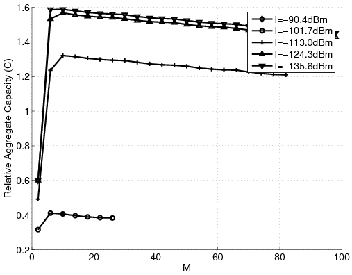
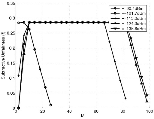
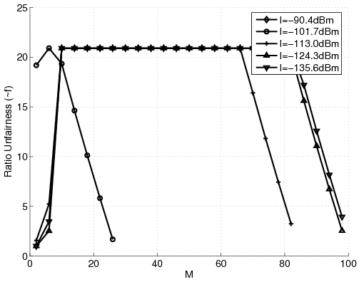
Figure 1: Results for different number of stations with g = -40dB and varying I in the new problem. (a) Aggregate Relative Capacity. (b) Subtractive Unfairness. (c) Ratio Unfairness.
Using the sequence gi, we analyze the effects of different parameters on the solution. The analysis is conducted in this way; first we show the values of C, the aggregate relative capacity. Then, we analyze the unfairness measures f and [f\tilde].
The first experiment studies how selecting between different values of I and g affects the system while the number of stations changes from one to a hundred. It was shown in [9] that as g decreases the aggregate capacity increases. The interpretation for that effect was that decreasing g means that the system is less engaged with the majority and can allocate more resources to the "elite" station. It was argued that this is not practically an acceptable policy. Figures 1-(a) to (c) show that the new problem does not exhibit an event like that. Here, g has negligible effect on the aggregate capacity, partly because not many stations are treated at that low rate. Also, we see that with the new problem, the aggregate capacity does not drop vastly when M increases. For example, for g = -50dB, the new problem's aggregate capacity drops less than 0.1 when M goes from 1 to 100 (6.4% of the amplitude). At the same time the classical problem results in the relative drop in the aggregate capacity by 6 (75% of the amplitude) [9]. However, similar to the case of the classical problem, we see that increasing I decreases the aggregate capacity. It should be mentioned that the aggregate capacity of the new problem is almost one third of that of the classical problem and the difference increases vastly when g reduces. We argue that the high aggregate capacity of the classical problem does not mean that that system is in fact capable of producing that much revenue, because it is relying on one "elite" station which may not exist. The ratio unfairness of the new problem is less than one tenth of the classical problem and the gap increases as g reduces, because the classical problem becomes more partial.
 |  |
| (a) | (b) |
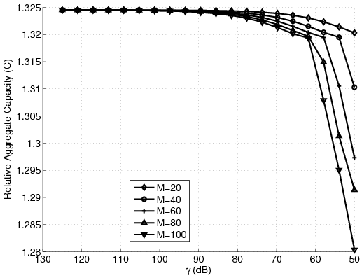
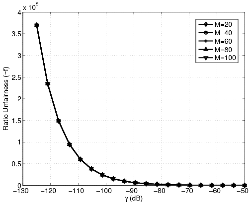
Figure 2: Results for different number of stations with varying g in the new problem. (a) Aggregate Relative Capacity. (b) Ratio Unfairness.
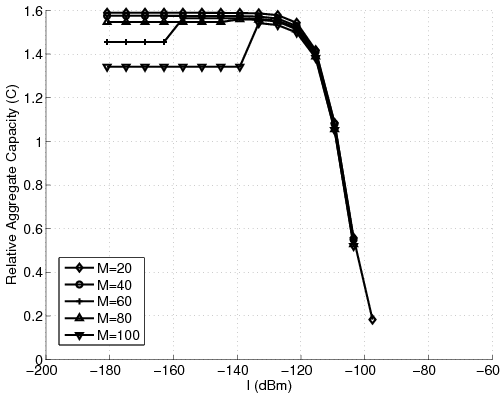
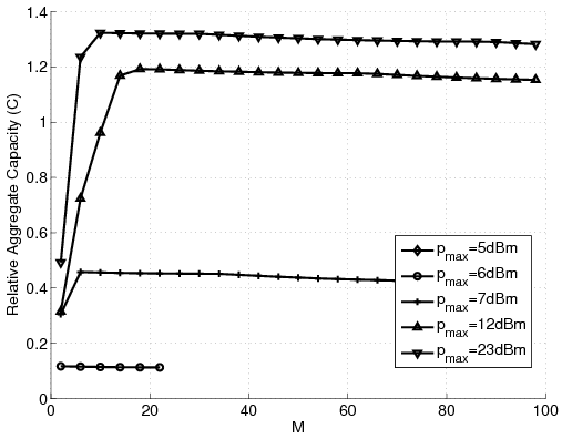
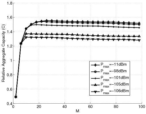
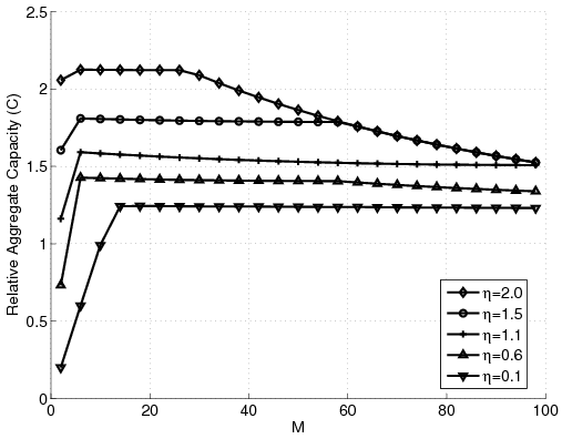
Figure 3: Aggregate relative capacity in the new problem for different number of stations. (a) Varying I. (b) Varying pmax. (c) Varying Pmax. (d) Varying h.
Analyzing the case when g is zero, meaning there is no minimum guaranteed quality of service, we observe that the ratio unfairness increases to more than ten thousand, still one thirtieth of the classical case [9]. Figure 2 shows the effects of varying g. Here, we see that having g > -80dB the ratio unfairness becomes acceptable. Also, note that the number of stations has no effect on the ratio unfairness curves. Looking at the subtractive unfairness curves we observe that they are independent of the number of the stations, too. Figure 3-(a) shows how varying I affects the solution. Note how increasing I over -130dB drops the aggregate capacity curves to great extents. Again, in contrary to the classical case [9], the unfairness curves are independent of the number of the stations. Figures 3-(b) and 3-(c) show the effects of pmax and Pmax on the solution. Finally, Figure 3-(d) shows that decreasing h decreases the aggregate capacity, because the maximum capacity of each station is then limited. However, as expected, reducing h decreases the unfairness. Note that because of shortage of space the unfairness curves are not shown here. We refer the interested reader to [12].
To have a better insight about the new problem and its benefits over the classical problem an experiment was carried out to compare their behavior in the long-run. We assume that M stations are in a cell. Here M=5 is selected to make a better visualization. Each station is first randomly put in the cell. We assume that each station is a pedestrian. Hence, the movements of each station is modeled as a random walk. Denoting the position of the i-th station at time t as [(x)\vec]i(t) we calculate, [(x)\vec]i(t+dt)=[(x)\vec]i(t)+s[
| ]Tvdt. Here, q is a uniform random variable in the interval [0,2p] and v equals 5Km/h [13]. Also, s is a uniform random variable in the interval [0,1]. Here, we assume that no station leaves the cell. Also, we do not consider the ones that enter it. Hence, at each time epoch we normalize the vectors [(x)\vec]i(t) which leave the cell as, R||[(x)\vec]i(t)||-1[(x)\vec]i(t). In this way, the boundaries of the cell are assumed to reflect the stations. Now, selecting values of T=20s and dt=0.1s and generating sequences of the random variables q and s, we produce the pattern of movement of the stations. This pattern of movement results in different values of gi over time. Clearly, as a station gets far from the antenna the respective value of gi decreases and vice versa. Now, we analyze the result of solving the classical and the new problems in this situation. First note that while the system is sampled every 100ms the solutions take only 7ms and 36ms for the two problems, respectively. This means that the system is only being utilized 7% and 36% of the time for the classical problem and the new problem, respectively.
Comparison shows that the classical problem tends more to force stations to have rapid increase and decreases in the power. That's mainly because the classical problem tries to devote almost all resources to the station which is the closest to the base. As the stations move around they compete for this occasion. Comparing the resulting capacities of different cells over time reveals a similar pattern. The curves for the classical problem show that the stations are mostly oscillating between two situations of minimum capacity and a very high one. This is another clue into the classical problem's tendency to serve one station with a very high capacity. On the other hand, the new problem keeps the capacity of different cells between the two specified bounds. The interesting part is that the capacity of none of the stations is ever squeezed down to the minimum guaranteed limit (this may not always be true). Also, in the classical problem we observe a very oscillating trend of capacities (the interested reader is referred to [12] for more extensive discussions).
 |  |
| (a) | (b) |
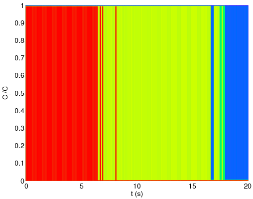
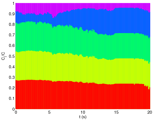
Figure 4: Capacity share of different stations over time shown by different colors. (a) Classical problem. (b) New problem.
To better understand the difference between the two problems we compare the values of capacity share of different stations in the two solutions. As the capacity shares of the stations for each problem at any moment sum to one, we show their values using bar graphs (see Figure 4). Here, each color shows the capacity share of one station over time. As anticipated, the classical problem tends to produce its revenue from one station at any moment. We can see in Figure 4-(a) that almost all bandwidth at each moment is devoted to the closest station. On the contrary, the new problem only increases its dependency upon each station as it gets closer. In this way, while the system is looking for more possible revenue, is it not demanding stations to transmit at bandwidths which are out of the range determined by g and h. Also, no station is ever left with the minimum guaranteed capacity. On the contrary, we see that the classical problem very frequently serves stations at the lowest possible capacity.
Comparing the aggregate capacity of the two solutions, we find out that the interesting results of the new problem have the cost of having almost half aggregate capacity. On the other hand, comparing the unfairness values shows that the new problem is massively more fair (almost one hundred times more in ratio). Given this experiment, and the other results presented in this paper and also in [12], we conclude that the new problem leads to a more practical solution to the QoS problem compared to the classical formulation.
4 Conclusions
In this paper we showed that adding a maximum capacity constraint to the classical QoS problem limits the unfairness of the system. Also, it was shown that this constraint only increases the computational cost from O(M2) to O(M3). The analysis of the new problem was carefully carried out and using the tools and concepts developed for the classical problem an algorithm for solving the new problem was proposed. Then, based on extensive experimental results, the performance of the new system was analyzed and was also compared with the classical one. To give a better insight about the new problem and its benefits over the classical one, two scenarios were discussed. First, using the same set of parameters, plus the new maximum bound for the proposed problem, the solutions given by the two problems were compared. It was observed that, in accordance to the available results, classical problem demands one station to transmit at a very high rate. Then, a dynamic case was investigated. The experiment revealed that the classical problem separates the set of the stations into all but one which are served at minimum possible rate and one "elite", the closest station, which is served at the most possible capacity, allowed by the constraints. The new problem, on the other hand, was observed to distribute resources evenly between stations and also to reasonably increase reliance on the stations when they get closer. Based on all evidence it was suggested that the application of the new problem leads to a more practical solution with an affordable increase in the computational cost.
Acknowledgement
The research of A. S. Alfa is partially supported by a grant from NSERC. We thank Mr. Haitham Abo Ghazaleh for guiding us to the data for the simulation part. The first author wishes to thank Ms. Azadeh Yadollahi for her encouragement and valuable discussions. We also appreciate the respected anonymous referees for their constructive suggestions.
References
- [1]
-
R. Knopp and P. Humblet, "Information capacity and power control in
single-cell multiuser communications," in 1995 IEEE International
Conference on Communications, Seattle, 1995, pp. 331-335.
- [2]
-
S. V. Hanly and P. Whiting, "Information-theoretic capacity of multi-receiver
networks," Telecommunication Systems, vol. 1, pp. 1-42, 1993.
- [3]
-
W. Lee, "Estimate of channel capacity in rayleigh fading environment,"
IEEE Transactions on Vehicular Technology, vol. 39 (3), pp. 187-189,
1990.
- [4]
-
S. V. Hanly and D. Tse, "Power control and capacity of spread-spectrum
wireless networks," Automatica, vol. 35 (12), pp. 1987-2012, 1999.
- [5]
-
S. Kandukuri and S. Boyd, "Simultaneous rate and power control in multirate
multimedia CDMA systems," in IEEE Sixth International Symposium on
Spread Spectrum Techniques and Applications, NJIT, NJ, 2000, pp. 570-574.
- [6]
-
S.-J. Oh, D. Zhang, and K. M. Wasserman, "Optimal resource allocation in
multi-service CDMA networks," IEEE Transactions on Wireless
Communications, vol. 2, pp. 811-821, 2003.
- [7]
-
S. A. Jafar and A. Goldsmith, "Adaptive multirate CDMA for uplink throughput
maximization," IEEE Transactions on Wireless Communications, vol. 2,
pp. 218-228, 2003.
- [8]
-
S.-J. Oh and A. C. K. Soong, "QoS-constrained information-theoretic sum
capacity of reverse link CDMA systems," IEEE Transactions on
Wireless Communications, vol. 5 (1), pp. 3-7, 2006.
- [9]
-
A. Abadpour, A. S. Alfa, and A. C. Soong, "Closed form solution for
QoS-constrained information-theoretic sum capacity of reverse link
CDMA systems," in Proceedings of the second ACM Q2SWinet 2006,
Torremolinos, Malaga, Spain, 2006, pp. 123-128.
- [10]
-
D. J. Goodman and N. B. Mandayam, "Power control for wireless data,"
IEEE Personal Communications Magazine, vol. 7, pp. 48-54, 2000.
- [11]
-
D. J. Goodman, Wireless Personal Communications Systems. Readings, Massachusetts: Addison-Wesley Wireless
Communications Series, 1997.
- [12]
-
A. Abadpour, A. S. Alfa, and A. C. Soong, "Information-theoretic sum capacity
of reverse link CDMA systems in a single cell, a more realistic approach,"
Electrical & Computer Engineering Department, University of Manitoba,
Winnipeg, Canada, Tech. Rep., 2006.
- [13]
-
B. Jabbari and W. F. Fuhrmann, "Teletraffic modeling and analysis of flexible
hierarchical cellular networks with speed-sensitive handoff strategy,"
IEEE Journal on Selected Areas in Telecommunications, vol. 15 (8), pp.
1539-1548, 1997.
File translated from
TEX
by
TTH,
version 3.72.
On 29 Nov 2007, 13:30.
|