A New Parametric Linear Adaptive Color Space and its PCA--based Implementation
A New Parametric Linear Adaptive Color Space and its PCA-based Implementation
A. Abadpour and S. Kasaei
Sharif University of Technology
abadpour@math.shrif.edu and skasaei@sharif.edu
Abstract
In many vision applications, color is an important cue that must
be applied very fast. In this paper, after giving a brief review
on 12 different standard color spaces, the proposed
parametric linear adaptive color (PLAC) space is defined. A
color-based segmentation process is performed on these color
spaces. Experimental results show that the PLAC can be applied
at least three times faster than the standard color spaces. In
addition, with 10% higher distinguishing power, the PLAC
shows the fail rate of half as much of the standard spaces. The
best advantage of the PLAC is its ability to remove the entire
background in 75% of the objects; compared to the low 1.69%
of the standard spaces. As the PLAC needs the semiautomatic
tuning stage, the proposed PCA-PLAC method is introduced
encapsulating the advantages of the PLAC with less required user
supervision even than the standard color spaces. The results show
the superiority of the proposed color spaces, while the PCA-PLAC
even outperforms the PLAC.
Keywords: Adaptive color space, principle component
analysis, color segmentation, color perceptions, color attributes.
Color is the way the human visual system (HVS) perceives a
part of the electromagnetic spectrum approximately between
380nm and 780nm. A color space is a method to
code a wave in this domain.
Although due to practical reasons, RGB color space is widely
used in the science and technology, when dealing with natural
images it suffers from high correlation between its components:
0.78 for rBR, 0.98 for rRG and 0.94 for
rGB [1]. Also the RGB color space has proved to be
psychologically not intuitive [2] in the way that
human has problems imagining pure colors Red, Green and Blue
as defined in RGB. Also, RGB is perceptually
non-uniform [2,3] because the correlation between the
perceived difference of two colors and the Euclidian distance in
RGB space is too low.
Different color spaces proposed in the literature with different
aims, could be informally categorized into three major categories
of HVS-based (including RGB; opponent and phenomenal color
spaces), application specific, and CIE color spaces for
better understanding [4].
In the late 19th century, Ewald Hering proposed the
opponent color theory [4]. The relating color space was
modelled by different researchers like Judd, Adams,
Hurvich, Jamson and Guth [4],
Another One is an excellent color space proposed by
Ohta [5] as a very good approximation of the
Karhunen-Loeve transformation of the decorrelated RGB
space (The color spaces is sometimes called I1I2I3):
ì ï ï ï í
ï ï ï î
I1=
1
3
(R+G+B)
I2=
1
2
(R-B)
I3=
1
4
(2G-R-B)
(1)
Phenomenal color spaces, using attributes of hue and
saturation (based on Newton's color circle) have
been proved to be the most natural way to describe human sense of
color [2]. There exists many different color models of
this category defined in the literature; such as the HSI
(2) [6] and HSV
(3) [7] [8]. Although the phenomenal
color spaces are very intuitive, but they have inherited the
device-dependent tendency from the mother space RGB along with
a hue discontinuity around 2p, and the main shortcoming of
non-uniform perception.
ì ï ï ï ï í
ï ï ï ï î
I=
1
3
(R+G+B)
S=1-
min(R,G,B)
I
H=cos-1
æ è
1
2
[(R-G)+(R-B)]
Ö
[`((R-G)2+(R-B)(G-B))]
ö ø
(2)
ì ï ï ï ï ï ï í
ï ï ï ï ï ï î
V=max(R,G,B)
S=
max(R,G,B)-min(R,G,B)
max(R,G,B)
H=
ì ï í
ï î
h,B £ G
2p-h,B > G
h=cos-1
æ è
1
2
[(R-G)+(R-B)]
Ö
[`((R-G)2+(R-B)(G-B))]
ö ø
(3)
Application specific color spaces are those invented for special
commercial purposes including the spaces used in printing systems
(CMYK (4)) [9], television systems (YUV
(5) [10], YIQ (6) [11],
YCbCr (7) [12]) and photo systems (YCC).
These color spaces are quite nonintuitive and perceptually
non-uniform.
ì ï ï ï ï ï ï ï í
ï ï ï ï ï ï ï î
K=min(
~
C
,
~
M
,
~
Y
)
C=
~
C
-
~
K
1-
~
K
M=
~
M
-
~
K
1-
~
K
Y=
~
Y
-
~
K
1-
~
K
~
C
=1-R,
~
M
=1-G,
~
Y
=1-B
(4)
ì ï í
ï î
Y=0.30R+0.59G+0.11B
U=-0.15R-0.29G+0.44B
V=0.62R-0.52G-0.10B
(5)
ì ï í
ï î
Y=0.30R+0.59G+0.11B
I=0.60R-0.28G-0.32B
Q=0.21R-0.52G+0.31B
(6)
ì ï í
ï î
Y=0.30R+0.59G+0.11B
Cb=0.56(B-Y)
Cr=0.71(R-Y)
(7)
In 1931, CIE laid down the CIE1931 standard to make a resolution
for the device-dependent tender of RGB color space and others
spaces based on it. The standard leads to the standard CIE-XYZ
as a color space describing the average human observer
(8). In 1976, CIE proposed two color spaces named
officially as CIE-Lu*v* (9) and CIE-La*b*
(10) whose main goals were to provide a perceptually
uniform space, of course later it was proved that the
CIE-Lu*v* is not entirely uniform [13]. The newly
defined color space CIE-L*HoC* (11) is the polar
version of the CIE-La*b* [9].
ì ï í
ï î
X=0.61R+0.17G+0.20B
Y=0.30R+0.59G+0.11B
Z=0.00R+0.07G+1.12B
(8)
ì ï ï ï ï ï í
ï ï ï ï ï î
L*=116f(
Y
Y0
)
u*=13L*(ú-úWhite)
v*=13L*(\¢v-\¢vWhite)
ú=
4X
X+15Y+3Z
\¢v=
9Y
X+15Y+3Z
(9)
ì ï ï ï í
ï ï ï î
L*=116f(
Y
Y0
)
a*=500(f(
X
X0
)-f(
Y
Y0
))
b*=500(f(
Y
Y0
)-f(
Z
Z0
))
(10)
ì ï ï ï í
ï ï ï î
L*=116f(
Y
Y0
)
Ho=tan-1
æ è
b*
a*
ö ø
C*=
Ö
a*2+b*2
(11)
Where f(x) in (9) and (10) and (11) is
the function:
In many applications of vision , color is an important cue
(because it is robust towards changes in orientation and scaling
and can well tolerate occlusion), but it is often computationally
expensive. For example, the RoboCup games are held in a
field officially defined as "a square with green carpets
and white walls in which two teams of four or five completely
black robots are trying to kick a red ball toward two goals
colored in blue and yellow respectively" [14]. In this
atmosphere, vision is the essential tool to recognize objects and
is based on the color diversity. For a soccer player robot, going
towards the ball at about 2m/s velocity, processing 16
frames per second results in about 30 mm error in each frame
(500mm error in any second.), which is a real shortcoming.
This proves the need for an enough accurate algorithm that is
performed fast enough.
There are a few color space comparison articles in the literature.
A recent work [15] considers the effects of color space
selection on the skin detection performance, reporting that non of
the 8 color spaces of normalized RGB (NRGB also called NCC),
CIE-XYZ, CIE-La*b*, HSI, spherical coordinate transform
(SCT), YCbCr, YIQ, and YUV seemed to respond better than
others. Another paper [16] investigates 5 color spaces
including RGB, YIQ, CIE-La*b*, HSV, and Opponent color,
and experimentally compares them in terms of human ability to
produce a given color by changing the coordinates in a given color
space, the paper does not concern the segmentation.
The first step towards recognizing an object in a captured image
is to distinguish it from the background. Although different
segmentation methods have been proposed (For two new methods see
[17,18].), but the accuracy and speed of such
algorithms greatly depend on the selection of the feature vector
describing the color information.
An object-in-image segmentation process is meant to detect
the area containing the object; and to extract the edges between
the object and the background. When using such method, the result
may include some parts of other objects. This is sometimes
inevitable but for performance reasons, an accurate segmentation
task is preferred which completely removes the background.
It must be denoted that segmentation processes, that work on color
information of each pixel independent of the neighborhood
information are more preferred for their byte-steam tender
and algorithm speed.
Spotting colors concerns with the accuracy with which objects of a
specific single color can be identified in a complex
image [19].
Although many color-based object recognition methods has been
proposed [20,21,22,23] but generally they work on
a multicolored object. For example Yullie [22]
proposed an algorithm for detecting street signs. The method uses
the relative appearance of the two colors in the signs. Algorithms
proposed by Ennesser [21] and
Funt [23] uses color-edge histograms for
recognizing a multicolored object.
Although many sophisticated methods for color space clustering
exist in the literature, but we selected a simple comparison
method, assuming that the selected color space is well-defined. A
recent work [24] uses 6 marginal values for the three
channels but proves that the common comparing operation is not
suitable for pipelining; it proposes the use of a lookup table
instead and reports the application of such method in a soccer
robot with 2MB of RAM. As the method needs a large mass of
memory and is slow and tedious when trying to learn another region
to the system, we limited the comparison to just one channel,
putting emphasize on proper color space selection but making the
whole operation faster.
The idea of reducing the color space dimension is
not a new idea; many researchers have reported benefits of
illumination coordinate rejection (For an example see [15], for further information see [25]).
The principle component analysis (PCA) [26] (For
more information see [27,28].) is widely used in signal
processing, statistics, and neural networks. In some areas, it is
called the (discrete) Karhunen-Leove transform (in
continuous case) or the Hotelling transform (in discrete
case).
The basic idea behind the PCA is to find the components s1¼sn, so that they explain the maximum amount of variance
possible by n linearly transformed components. By defining the
direction of the first principal component, say w1, by (13), the PCA can be represented in an intuitive way [26].
w1 = arg
æ è
max
\sb | w |=1
é ë
E { (wT x )2 }
ù û
ö ø
(13)
Thus, PCA is the projection of the data on the direction in
which the variance of the projection is maximized. Having
determined the first k-1 principal components, wk is
determined as the principal component of the residual stated
as [26]:
The principal components are then given by si=wiT x [26].
In practice, the computation of wi can be simply accomplished
using covariance matrix C = E{ (x- [`x]) (x- [`x])T }.
The wn is the eigenvector of C corresponding to the nth
largest eigenvalue [26].
The basic goal in PCA is to reduce the data dimension. Thus, one
usually chooses n << m. Indeed, it can be proven that the
representation given by PCA is an optimal linear dimension
reduction technique in the mean-square sense. Such a reduction in
dimension has important benefits. First, the computational
overhead of the subsequent processing stage is reduced. Second,
noise can be reduced, as the data not contained in the n first
components may be mostly due to noise [26].
A simple color spotting task is assumed as discussed in section
1.3 and a new parametric linear
adaptive color (PLAC) space is introduced that performs the
task more accurately and more robust compared to 12 standard
color spaces. As PLAC needs tedious tuning job, a new
Principle Component Analysis Based Parametric Linear
Adaptive Color PCA-PLAC space is introduced that encapsulates
the promising results of PLAC with a tuning method even easier
than the standard color spaces'.
Although any standard color space is defined as a function
G:R3® R3, in this paper we face each channel of a
color space independently. So we are concerned to perform the
classification according to a function X:R3® R. In
order to comply with notions of (17) and (21),
the discrimination function is defined as:
fXC,T(
®
c
)=
ì ï í
ï î
1,|X(
®
c
)-C| £ T
0,else
(16)
Where X(·) is the function producing one of
the channels of a selected color space out of the coordinates of
[c\vec] in RGB space.
Most of the standard color spaces suffer from the disadvantageous
fixed structures that makes them inefficient in treating special
odd-shaped loci in the color space. This was the main motivation
for defining the parametric linear adaptive color (PLAC)
space formulated in (17) with 5 user-selected parameters
ar,ag,ab,C,T.
ì ï ï ï ï ï í
ï ï ï ï ï î
far,ag,ab,C,TPLAC(
®
c
)=
ì ï í
ï î
1,|[(a)\vec]T[(c)\vec]-[(C)\tilde]| £ [(T)\tilde]
0,else
~
C
=Sax < 0ax+C
S|ax|
255
,
~
T
=T
S|ax|
255
®
a
=
æ ç
è
ar
ag
ab
ö ÷
ø
T
(17)
PLAC is a 1-D color space; in contrast with the ordinary 3-D
and 4-D color spaces.
3.3 Principle Component Analysis-Based Parametric Linear
Adaptive Color Space
As the tuning phase of PLAC needs massive user work, a new color
space named as principle component analysis-based parametric
linear adaptive color (PCA-PLAC) space is also introduced.
Rather than the numerical parameters tuned by the user in PLAC
and other color spaces, PCA-PLAC extracts the information from
the scene. When trying to use PCA-PLAC, one must give a
rectangle of the desired segment to the algorithm (Let's call the
region as R.). By forming the 3×A (A is the area of
R) matrix S containing the RGB values of all pixels in R ,
the vector [(h)\vec] is computed by row averaging of S to give
E[c\vec] Î R{[c\vec] } as a 3×1 vector. This vector
is used to produce the matrix D as the center oriented version
of S . The eigenvalues of the matrix C=DTD are computed and
the eigenvector corresponding to the largest eigenvalue is
selected to be [v\vec] .
The reconstruction error(RE) of a point regarding to the
region R is defined as (18) in which smaller values
shows more tendency. in (18), á[v\vec]ñis a
custom norm function defined in (19). The marginal
reconstruction error is computed as (20) and a tolerance
is asked from the user (l). The classification function
for an arbitrary point is defined in (21).
eR(
®
c
)=e[v\vec], [(h)\vec](
®
c
)=á \acute
®
v
[
®
c
-
®
h
]
®
v
-[
®
c
-
®
h
]ñ
(18)
á
®
v
ñ =
1
N
Si=1N|vi|
(19)
~
e
R
=argc Î R{P(eR(
®
c
) < e) > 0.95 }
(20)
fR,lPCA-PLAC(
®
c
)=
ì ï í
ï î
1,eR(
®
c
) £ l
~
e
R
0,else
(21)
It must be emphasized that although PCA-PLAC needs user to draw
a rectangle on the selected object, there is only one
user-selected parameter to be tuned in PCA-PLAC in contrast with
the 5 parameters in PLAC. It is worth mentioning that tuning
PCA-PLAC is more intuitive compared to tuning PLAC.
To find out the repeatability of PCA-PLAC, the correlation
between different results of spotting one object was computed as
(22), along with a parameter showing the range of the
tolerance in different tests on the same object as (23).
The 12 different color spaces under investigation are RGB,
CMYK, HSI, I1I2I3, CIE-La*b*, CIE-L*HoC*,
CIE-Lu*v*, CIE-XYZ, YCbCr, YIQ and YUV. According to
the categorizes of color spaces declared in section
1.1, There are four HVS-based, four
application-specific, and four CIE color spaces involved in this
study.
For more convenience all channels were considered as subsets of
[0... 255]3 and all singular point were defined to correspond
to zero value in the corresponding channels.
The objects in the sample image (See figure 1)were
indexed and their areas were calculated by manual segmentation
with repeatedly use of magic select tool in Adobe
Photoshop. To test the performance of spotting in the
pre-described standard color spaces, after computing the
representation of the sample image in 12 color spaces (37
channels), answers to the following questions were inspected in
each of the 37 channels for
each of the 8 objects:
How much is the most percentile of the object area when it is
cut out of the image with the best-selected set of parameters?
(Q1 Î [0 ... 100])
When trying to answer the first question, is the background
removed completely, without considerable intrusion? (Q2 Î {0,1 } mapped to [0 ... 100] in statistics.)
Also a zero-one fail rate parameter was defined, showing
the situations where the method is unable to distinguish the
border of the object. The answers to these questions were
acquired and statistically analyzed.
The tests were performed by a subject with 3 years expertise
on such segmentation tasks. User was using a graphic user interfaces(GUI) developed in
MATLAB 6.5 with scroll bars for tuning parameters (C,T
in standard color spaces, ar, ag, ab , C, and T in
PLAC and l in PCA-PLAC). He was looking at the
original image and the spotted image in two aside windows.
Experimental results are shown in section 4.2 and
section 4.3 compares PLAC, PCA-PLAC, and
standard color spaces.
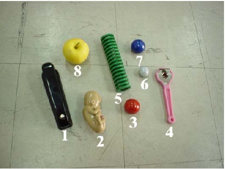
The sample image used in spotting test were taken from 8 objects
(Stapler, Infant, Red Ball, Tin
Opener, Spring, White Ball, Blue Ball, and
Apple) with different colors put on a smooth surface in the
daylight by a digital camera (Figure 1).
Figure 1: An image taken from eight objects with different
colors.
All algorithms were developed in MATLAB 6.5 with highly
optimized code, on an 1100 MHZ Pentium III personal
computer with 256MB of RAM.
Answers to the predefined questions were acquired in 37 channels
of the 12 color spaces (The table was too large to be printed in
this paper), also in PLAC (Table 1) and PCA-PLAC
(Table 2). Tests on the 8 objects were performed 5
times for each object in PCA-PLAC and the average values of all
dij in different tests on the same object were computed
as C along with the average value of all [(dl)\tilde] as [`([(dl)\tilde])] (Table
2). Table 3 compares fail rate, [`(Q1)]
, dQ and [`(Q2)] of the 37 channels, PLAC and
PCA-PLAC.
Table 1: Spotting results in PLAC.
1
2
3
4
Q1
86.1
95.2
72.2
56.8
Q2
100
0
100
100
5
6
7
8
Q1
67.8
-
82.5
99.9
Q2
100
0
100
100
Table 2: Spotting results in PCA-PLAC.
[`Q]1
dQ1
[`Q]2
[(dl)\tilde]
C
1
95
4.73
100
19
96.3
2
94.2
5.67
100
17
93
3
88
5.96
100
66
93
4
66.2
3.86
100
17
94.3
5
91.2
4.16
100
6
96.3
6
48.6
8.56
0
31
71.6
7
74.8
5.26
100
50
93.2
8
99.4
0.80
100
36
98
Average
82.17
4.88
87
30.25
92
Std. Dev.
16.78
2.19
30
19.36
8.94
Table 3: Comparison of results in standard color spaces,
PLAC and PCA-PLAC.
Investigating the Average and standard deviation of the spotting
results in standard channels is insightful. Of course the average
value of Q1 for most channels is higher that 50% but the
standard deviation of channels is too high (42.47%) which shows
that the method may act poor likely. Of course it must be
emphasized that in 73 tests the method was unable to find a
reasonable portion of the object or to distinguish the boarder
line, which leads to the desperate fail rate of 24.66%.
Over the stimuli the situation is even worse. It is clear that
spotting method's success in standard color spaces entirely
depends on the object. The best results have been recorded for the
apple, the red ball, the spring, the
blue ball and the stapler, which all make distinct
loci in the color spaces. The worst result has been captured for
the white ball, because it is very similar to the
background in color scheme.
In the 37*8=296 attempts made for cutting the desired object out
of the background, only 5 were successful to clear the entire
area, which gives the poor mathematical expectation of 1.69%.
This event is also very much depending on the subject, as 3 out
of the 5 has happened on the 7th object.
In table 1 it is clear that in 6 out of 8 attempts,
PLAC was successful to remove the entire background, which gives
the hopeful result of 75%. This measure is 87% for
PCA-PLAC as shown in table 2.
PLAC has failed to recognize the object in 12.5% of tests,
which is half the fail rate of standard methods, having in mind
that PCA-PLAC has never failed.
The expectation result of Q1 in PLAC, is 70.06% with
standard deviation of 31.68% in contrast with the average of
61.03% and standard deviation of 42.27% in standard color
spaces, showing about 10% better results with a smaller
standard deviation when comparing PLAC to standard color spaces,
making hope that PLAC responds uniformly in the stimuli range.
Table 2 shows even better results for PCA-PLAC
compared to PLAC. The surprising result of 82% expectation
value with variance of less than 5% for Q1 and 87%
expectation for Q2 when l has changed about 30%
shows the robustness of PCA-PLAC. It must be emphasized that the
average correlation is more than 90%.
It must be emphasized that as the two proposed PLACs are 1-D
color spaces, their computation time is at least three times less
than ordinary 3-D color spaces. Of course compared to the
sophisticated hue-saturation based color spaces, which use
complicated functions, the performance is far better. Also the
PLAC and PCA-PLAC are very much appropriate for analog
implementation by ordinary circuitry.
The clear disadvantage of PLAC is the tedious tuning job, which
reduces its repeatability and needs supervision of human observer,
a shortcoming that has been removed in PCA-PLAC. It is easy to
see that PCA-PLAC needs only one parameter to be tuned by the
user in contrast with the two parameters in standard spaces and
five parameters in PLAC, Also user has no intuition when setting
ar, ag,ab,C,T parameters in PLAC in contrast with the
meaningful l parameter in PCA-PLAC.
PCA-PLAC has appeared surprising to gain Q1=46.8% for the
peculiar 6th object, where all other methods, even the PLAC
have failed.
performance of 12 standard color spaces was considered in this
study and two measurements along with a fail rate were studied in
their respective channels when spotting homogenous regions in a
test image containing 8 different colored objects. The
measurements concerned the maximum percent of distinguishing power
and the background removal ability of each channel for each
object. Two color spaces PLAC (parametric) and PCA-PLAC
(PCA-based) were proposed and the same tests were performed on
them along with the repeatability test on the PCA-PLAC.
Experimental results showed that rather than the first 6
channels (R,G,B,C,M,Y), the PLAC and PCA-PLAC
gained lower fail rates. There were a few channels with the
average distinguishing power higher than the PLAC and only one
channel better than the PCA-PLAC, but the average result of both
of them was much higher than the standard color spaces. Also, the
standard deviation of the distinguishing power in the PLAC was
higher than all others while the results in the PCA-PLAC were
even higher than the PLAC.
Acknowledgement
Hardware used in this study was provided by the Gait Lab.,
Biomechanics group, Mechanics school, Sharif
University of Technology. Authors wish to specially thank
Mrs. R. Narimani for her encouragement and invaluable help.
Ingeborg Tastl and Gunther Raidl,
"Transforming an analytically defined color space to match
psychophysically gained color distances,"
the SPIE's 10th Int. Symposium on Electronic Imaging: Science
and Technology, San Jose, CA, SPIE, vol. 300, pp. 98-106, 1998.
Y. Kanade Y. I. Ohta and T. Saki,
"Color information for region segmentation,"
Computer Graphics and Image Processing, vol. 13, pp. 222-241,
July 1980.
Garvey T.D. Weyl S. Tenenbaum, J.M. and H.C. Welf,
"An interactive facility for scene analysis research,"
Tech. Rep. 87, Stanford Research Institute, AI Centre, 1974.
J.D. Foley and A. Van Dam,
Fundamentals of Interactive Computer Graphics,
The System Programming Series, Addison-Wesley,, Reading, MA., 1982,
Reprinted 1984 with corrections.
Nuas M. Ledley, S. and T. Golab,
"Fundamentals of true color image processing,"
Proceedings of 10th International Conference on Pattern
Recognition, Atlantic City, pp. 791-795, 1990.
Leonid V. Tsap Min C. Shin, Kyong I. Chang,
"Does color space transformation make any difference on skin
detection?,"
http://citeseer.nj.nec.com/542214.html.
William B. Cowan Micheal W. Schwarz and John C. Beaty,
"An experimental comparison of rgb, yiq, lab, hsv and opponent color
models,"
ACM Transaction on Graphics, vol. 6, 1987.
David E. Haynor Shijun Sun and Yongmin Kim,
"Semiautomatic video object segmentation using snakes,"
IEEE transaction on circuits and systems for technology, vol.
13, 2003.
F. Ennesser and G. Medioni,
"Fidning waldo, or focus of attention using local color
information.,"
IEEE Trans. on Pattern Analysis and Machine Intelligence, pp.
805-809, 1995.
Snow D. Yuille, A.L and M. Nitzberg,
"Signfinder:using color to detect, localize and identify
informational signs,"
Int. Conf. on Computer Vision ICCV98, pp. 629-633, 1998.