Principal Color and Its Application to Color Image Segmentation

Arash Abadpour ¹ and Shohreh Kasaei ²
¹ Mathematics Science Department, Sharif Univ. of Tech., Tehran, Iran, email: abadpour@math.sharif.edu
² Computer Engineering Department, Sharif Univ. of Tech., Tehran, Iran, email: skasaei@sharif.edu

Abstract

Color image segmentation is a primitive operation in many image processing and computer vision applications. Accordingly, there are numerous segmentation approaches in the literature, something which can be misleading for a researcher who is looking for a practical algorithm. While many researchers are still using the tools which belong to the old color space paradigm, there are evidences in the research established in eighties that proper descriptor of color vectors should act locally in the color domain. In this paper, we use these results to propose a new color image segmentation method. The proposed method searches for the principal colors, defined as the intersections of the cylindrical representations of homogeneous blocks of the given image. As such, rather than using the noisy individual pixels, which may contain many outliers, the proposed method uses the linear representation of homogeneous blocks of the image. The paper includes comprehensive mathematical discussion of the proposed method and experimental results to show the efficiency of the proposed algorithm.

1 Introduction

In 1988, Klinker, Shafer, and Kanade presented a novel approach to measure the highlights in color images [1]. In that work, they developed a proper model for the reflected light from an arbitrary point of a dielectric object. In 1990, they applied their approach to color image understanding [2]. However, more than a decade passed since the idea was successfully incorporated into a practical algorithm. In 2003, without paying too much attention to the theoretical aspects, Cheng and Hsia used the principal component analysis (PCA) for color image processing [3]. Then, in 2004, Nikolaev and Nikolayev started the work again from the theory and proved that the PCA is a proper tool for color image processing [4]. The next necessary step had been introduced in 1991, when Turk and Pentland proposed their eigenface method [5], in a completely different context. There, they developed a novel idea which connected the eigenproblems in the color domain and the spatial domain together. Although, there is this rich theoretical background for the linear local models of color, it is quite common to see research procedures which are based on the old color space paradigm, even published in 2005. For a more comprehensive discussion of this topic refer to [6].

In different works, the authors have applied the PCA, and then the fuzzy PCA (FPCA), to many different color image processing tasks. The essential idea of those works, which was borrowed from the above-mentioned literature, is that homogeneous swatches in color images of nature produce thin cylinders in the RGB space. In this framework, fuzzy clustering is a proper tool for finding these structures [7]. This theory opens plenty of opportunities for efficient color image processing tasks. Interested readers can refer to [8,9] for two applications of this theory. Also, see [6] for more examples.

In the PCA framework, each color swatch is represented by a line, which passes through its expectation vector and is parallel to its principal direction. Although, it is proved that the lines representing similar materials lie on a unique plane [1], the theory neglects the (possibly virtual) intersection of these lines. A virtual intersection of a set of lines is a point very close to which almost all of them pass. In this paper, we empirically show that the lines representing similar materials do intersect and show that this intersection leads to a new technique for color image segmentation. We call this intersection point the principal color of the underlying material.

A review of the color image processing literature shows the huge amount of research dedicated to the basic primitives such as color image segmentation. This results in a vast variety of approaches with different motivations and tools. The reader is referred to [10,11] and the references therein for more details. Although, there are many available segmentation algorithms, no numerical criterion is standardized to give a reasonable comparison between the results of different approaches. In fact, the only globally-accepted, and referred to, factors are the elapsed time and the visual properness of the results. Furthermore, the utilization of many techniques includes many parameters which must be tuned by an expert. Failing to do the required tuning, may result in total or partial collapse of the method (see [12] as an example). In this paper, we compare the performance of the proposed method with that of an available approach which is based on the same theory [7] and show that the new method outperforms the previous one. For the comparison of that method with the available literature refer to [7].

The rest of this paper is organized as follows. Section II introduces the concept of principal colors and gives experimental cues for their existence. Then, it describes the proposed method to use principal colors to perform color image segmentation. Section III holds the experimental results and discussions and finally Section IV concludes the paper.

2 Method

Here, we propose an investigation, through which the existence of the principal colors could be empirically perceived. We emphasize that this empirical result has to be confirmed by theoretical investigation. We believe that the increasing number of research projects devoted to processing color images will pave the way to the formal approval of this theory, something which is outside the scope of this paper.

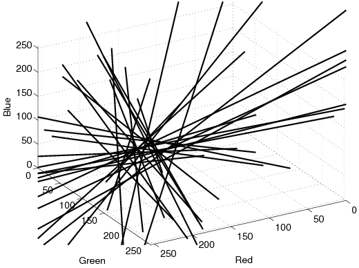
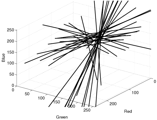
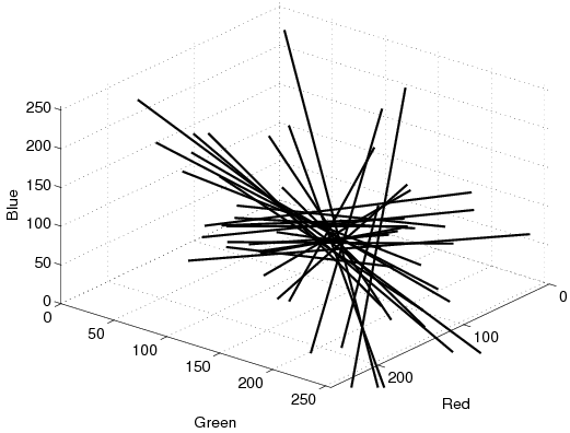
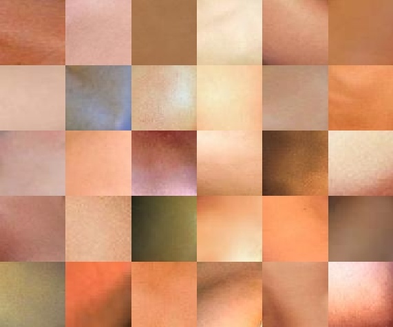
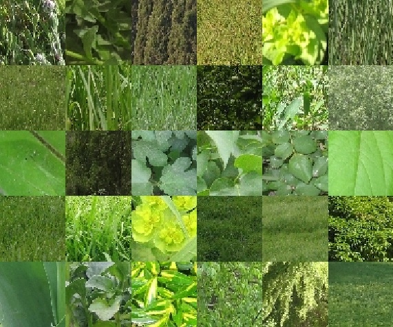
Figure 1 shows three sets of color swatches representing skin, sky, and leaf materials. Each set contains 30 images, each a 64×64 JPEG file with quality of 100. The skin samples are extracted from erotic images downloaded from free resources on the Internet. The sky and leaf samples are captured by a Cannon A60 digital camera in different times of the day and in different locations. For each category, the lines representing each single swatch are drawn in a common RGB space. Figure 2 shows these three sets of lines. Note that for each material, all the lines pass through a small region in the color space. We call this (virtual) intersection of the lines, the principal color of that material. Figure 3 shows the principal colors of skin, sky, and leaf extracted by the proposed method. Section II-A gives the mathematical details about the process which finds this point. Section II-B develops the idea further to include a set of fuzzy (or weighted) lines. Section II-D incorporates the principal color theory with the general clustering algorithm described in Section II-C to propose a new color image segmentation method.


(a)	(b)	(c)

Figure 1: Randomly selected samples representing three different materials. (a) Skin. (b) Sky. (c) Leaf.


(a)	(b)	(c)

Figure 2: Linear representation of the samples shown in Figure 1. (a) Skin. (b) Sky. (c) Leaf.


(a)	(b)	(c)

Figure 3: Principal color of the samples shown in Figure 1 extracted by the proposed method. (a) Skin. (b) Sky. (c) Leaf.

2.1 Finding the Closest Point to a Set of Lines

Assume that n lines of l₁,¼,l_n in \mathbbR^m are given. Also, assume that l_i is indicated by the two vectors [(h)\vec]_i and [(v)\vec]_i. As such, [(h)\vec]_i is a vector starting from the origin (with its head on l_i) and [(v)\vec]_i is the direction of l_i, satisfying ||[(v)\vec]_i||=1. Hence, the points on l_i occupy the set L_i Ì \mathbbR^m, which is defined as,

L_i=

ì
í
î

|l Î \mathbbR

ü
ý
þ

(1)

We assume that [(h)\vec]_i is perpendicular to [(v)\vec]_i ([(h)\vec]_i^T[(v)\vec]_i=0). If this condition is not met, [(h)\vec]_i is replaced with,

*
i

æ
è

t
i

ö
ø

(2)

The closest point to the n lines, l₁,¼,l_n, is the point [(x)\vec] Î \mathbbR^m which minimizes the following objective function,

D =

n
å
i=1

æ
è

,l_i

ö
ø

(3)

where, d([(x)\vec],l_i) is the distance from the point [(x)\vec] to the line l_i. Linear algebra shows that,

æ
è

,l_i

ö
ø

=||

æ
è

ö
ø

é
ë

T
i

æ
è

ö
ø

ù
û

||²,

(4)

which is simplified to,

æ
è

,l_i

ö
ø

æ
è

ö
ø

é
ë

I-

T
i

ù
û

æ
è

ö
ø

(5)

Substituting (5) in (3) gives,

D =

n
å
i=1

æ
è

ö
ø

é
ë

I-

T
i

ù
û

æ
è

ö
ø

(6)

From calculus we know that [13],

æ
è

ö
ø

+A^T

(7)

Hence,

¶D

n
å
i=1

é
ë

I-

T
i

ù
û

æ
è

ö
ø

(8)

Setting [(¶D)/(¶[(x)\vec])]=0 gives,

é
ë

I-

n
å
i=1

T
i

ù
û

n
å
i=1

(9)

Now, we will prove that the n×n matrix on the left hand side of (9), which we call U, is always non-singular, given that not all [(v)\vec]_is are parallel.

A theory in linear algebra states that, "if I+E is singular then ||E|| ³ 1, where ||·|| is a subordinate matrix norm" [14]. We will first prove this theorem. Assume that I+E is singular. Hence, there exists a non-zero vector [(x)\vec] satisfying (I+E)[(x)\vec]=[(0)\vec]. Thus, [(x)\vec]=-E[(x)\vec] or equivalently,

||E|| ³

||E

=1.

(10)

Thus, to prove that U in (9) is non-singular, it suffices to show that,

n
å
i=1

T
i

|| < n.

(11)

We prove (11) by showing that for any vector [(y)\vec] satisfying ||[(y)\vec]||=1, we have,

n
å
i=1

T
i

|| < n,

(12)

First, we know that for any two arbitrary m×1 vectors [(u)\vec] and [(v)\vec],

| £

æ
Ö

||²||

||²

(13)

Note that equality occurs for [(u)\vec]||[(v)\vec]. Thus, in the case discussed here we have |[(v)\vec]_i^T[(y)\vec]| £ 1, which results in,

n
å
i=1

T
i

|| £

n
å
i=1

T
i

|||

|| £

n
å
i=1

||=n.

(14)

Here, the equality happens only if all [(v)\vec]_is are parallel. Thus, ignoring this very especial case, (12) is proved, proving that the solution to (9) exists and is,

é
ë

nI-

n
å
i=1

T
i

ù
û

-1

n
å
i=1

(15)

Here, [(x)\vec] is the closest point to the n lines l₁,¼,l_n.

2.2 Finding the Closest Point to a Set of Fuzzy Lines

Assume that we are looking for the closest point to the set of n lines l₁,¼,l_n in \mathbbR^m. Also, assume that the importance of l_i is p_i ³ 0. This means that when composing the objective function, we will weigh satisfaction of l_i by p_i. Hence, as p_i grows, the importance of l_i in decisions grows linearly, and the vice versa. As such, we are looking for [(x)\vec] Î \mathbbR^m which minimizes,

n
å
i=1

p_id

æ
è

,l_i

ö
ø

(16)

Note that setting "i, p_i=1 converts (16) into (3). An analysis similar to the one performed in Section II-A reveals that [(x)\vec] is computed as,

é
ë

n
å
i=1

p_iI-

n
å
i=1

p_i

T
i

ù
û

-1

n
å
i=1

p_i

(17)

Again note that assuming "i, p_i=1 converts (17) into (15), as expected.

2.3 General Clustering Algorithm

Assume that the fuzzy set of n vectors [(x)\vec]₁,¼,[(x)\vec]_n in \mathbbR^m is given as [(X)\tilde]={([(x)\vec]_i;p_i)|i=1,¼,n}. Also, assume that a human observer has a perception of homogeneity for the subspaces of this space. For example, for m=3 every human being is able to think and argue about the homogeneity of a set of color vectors. Also, when considering lines in \mathbbR³, which are members of \mathbbR⁶, the meaning of homogeneity used here is the existence of a point which is very close to almost all of them. In many occasions, a homogeneous set may be parameterizable. For example, research shows that a homogeneous set of color vectors occupies a thin cylinder which will be described by two vectors. Similarly, a set of (virtually) intersecting lines may be parameterized by a single point. Thus, we assume that there is a function U that extracts this parametrization for the homogeneous fuzzy set [(X)\tilde]. As an example, if a homogeneous set in \mathbbR^m is defined as a sphere, the U function will be a fuzzy expectation operator. Also, for the cylindrical homogeneity, U will be the FPCA [7]. Having defined a description of a homogeneous set as f, there might exist a function Y which measures the distance from an arbitrary element to f. For the spherical example, the Y function is the Euclidean distance. Also, the Y function of the cylindrical homogeneity, is the linear partial reconstruction error (LPRE) distance proposed in [6].

Having proper dual functions U and Y, and a fuzzy set [(X)\tilde], an important problem is how to separate [(X)\tilde] into c homogenous clusters, where c is known. This problem is called the general clustering problem [7]. The special cases of this problem are the fuzzy C-means (FCM) [15] (in which the clusters are spherical) and fuzzy C-varieties (FCV) [16] (in which the clusters are subspaces). Other examples are Gath-Geva [17], fuzzy elliptotypes [18], Gustafson-Kessel [19], and FPCA-based clustering (FPCAC) [7] algorithms. Figure 4 shows the pseudo-code of an iterative solution to the general clustering problem. The interested reader is referred to [8] for the related mathematics and the proof of the convergence.

As shown in Figure 4, the algorithm first randomly initializes the clusters. Then, it iterates between computing the distance of each member to each cluster and then renewing each cluster according to the membership value of the realizations to it. The algorithm contains an important parameter of fuzziness [20], m, which is always more than unity. The general clustering algorithm enables the clustering of any kind of data, given that a proper distance function and its dual are available. In Section II-D we will give a distance function which searches a set of lines for lines passing through or getting very close to a common point. The distance function is then integrated into a novel color image segmentation procedure.

Aim: Clustering data according to the given model.

Inputs:

Appropriate distance function (Y and its dual U).

Set of realizations (X={[(x)\vec]₁,¼,[(x)\vec]_n}).

Number of clusters (c).

Fuzzyness (m).

Halting threshold (d).

Outputs:

Fuzzy membership values (p_ij).

c cluster descriptors (f₁,¼,f_c).

Method:

1 k=0 and randomize f₁,¼,f_c.
2 k=k+1.
3 D_ij=Y([(x)\vec]_i,f_j).
4 p_ij=D_ij^-1/(m-1)/å_k=1^cD_ik^-1/(m-1).
5 F_kij=p_ij.
6 f_j=U{([(x)\vec]₁;p_1j^m),¼,([(x)\vec]_n;p_nj^m)}.
7 if k=1, then goto 2.
8 d_k² = min_{1 £ p £ l-1}E_i,j{(F_pij-F_kij)²}.
9 if d_k > d, then goto 2, else return.

Figure 4: Pseudo-code of the general clustering algorithm [7].

2.4 Color Image Segmentation using Principal Colors

Assume that the H×W color image I is given. Also, assume that the integer c is given as the number of homogeneous segments that I should be split into. For now, assume that both H and W are divisible by 2ⁿ, where n is an integer larger than 2. It is clear that, using zero-padding or resampling, the same operation is applicable to any image. We propose to cut I into 2^-2nWH non-overlapping rectangular blocks of 2ⁿ×2ⁿ pixels.

In [6], the authors proposed a novel homogeneity criterion for color swatches. In that work, the LPRE criterion was compared to the Euclidean and Mahalanobis distances and its superiority was proven. As such, the non-homogeneity of the swatch i is defined as [6],

t(i)²=E_{[(c)\vec] Î i}

ì
í
î

æ
è

ö
ø

T
i

æ
è

ö
ø

||²

ü
ý
þ

(18)

Here, [(h)\vec]_i is the expectation vector of i and [(v)\vec]_i is the principal direction of i. Also, ||[(x)\vec]|| is the Euclidean length of the vector [(x)\vec]. We use t(i) < q to decide whether a swatch is homogeneous or not, where q is a constant threshold. Experiments show that q = 10 is a proper choice [6].

In the proposed segmentation method, from the 2^-2nWH blocks, those which are not homogeneous are deleted. For the remaining blocks, the PCA representations are saved as the m lines of l₁,¼,l_m, all in \mathbbR³. Now, the problem is to find c proper intersections of these lines. Using the notations of the general clustering algorithm (see Section II-C) each realization is a line in \mathbbR³ and the cluster model is a 3-D point. As such, the distance between the line l (denoted by [(h)\vec] and [(v)\vec]) and the point [(x)\vec] is defined as,

æ
è

ö
ø

=||

æ
è

ö
ø

æ
è

ö
ø

||².

(19)

In this framework, the dual function U is given by (17). Here, the fuzzy set is [(L)\tilde]={(l_i;p_i)|i=1 ¼,m}, where l_i is represented by [(h)\vec]_i and [(v)\vec]_i.

The general clustering algorithm results in a set of c points in \mathbbR³, where each point is the principal color of the respective cluster. Note that at the beginning of this process, the non-homogeneous blocks were removed. That was done because the principal direction of those blocks are not meaningful. Therefore, at this point, the process should assign each block to a cluster, even those that are not homogeneous enough. Also, note that the results of the general clustering algorithm is a set of fuzzy membership values for each block and each cluster. Thus, using a maximum-likelihood operator, each block is deterministically assigned to one of the clusters. By finding the distance of each omitted block to all clusters, the process assigns them to one of the computed clusters. The next step is to interpolate the assignment for all pixels. As each block is a 2ⁿ×2ⁿ swatch, performing bilinear double-sampling on the resulting index map, for n times, yields the desired segmentation. In practice, blocks of size 2^n₁×2^n₁ are used to find the clusters and then 2^n₂×2^n₂ blocks are examined to compute the index-map.

3 Experimental Results

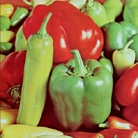
The proposed algorithm is developed in MATLAB 6.5, on a PIV 2600 MHz personal computer with 256 MB of RAM. All sample images used in this paper are 512×512 color images in JPEG format with quality of 100 (see Figure 5).


(a)	(b)	(c)

(d)	(e)	(f)

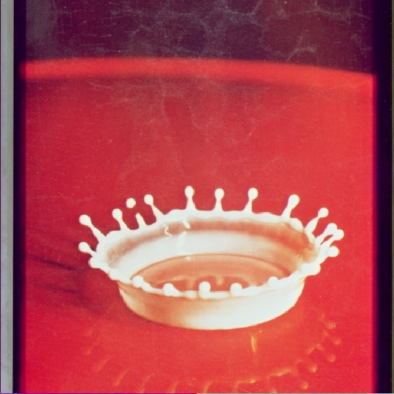
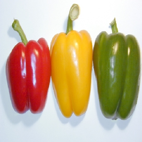
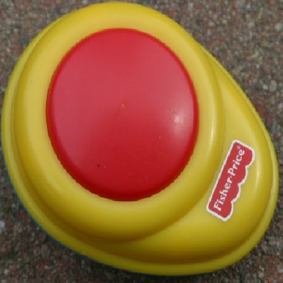
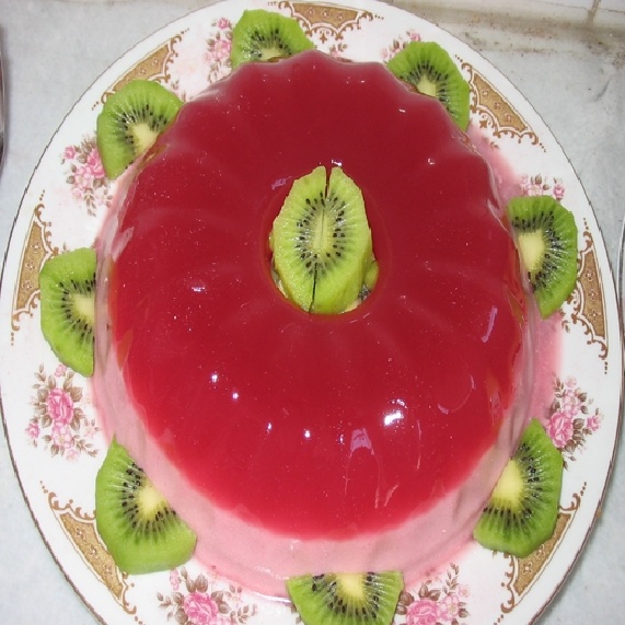
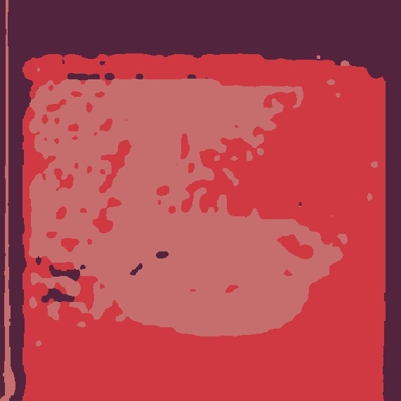
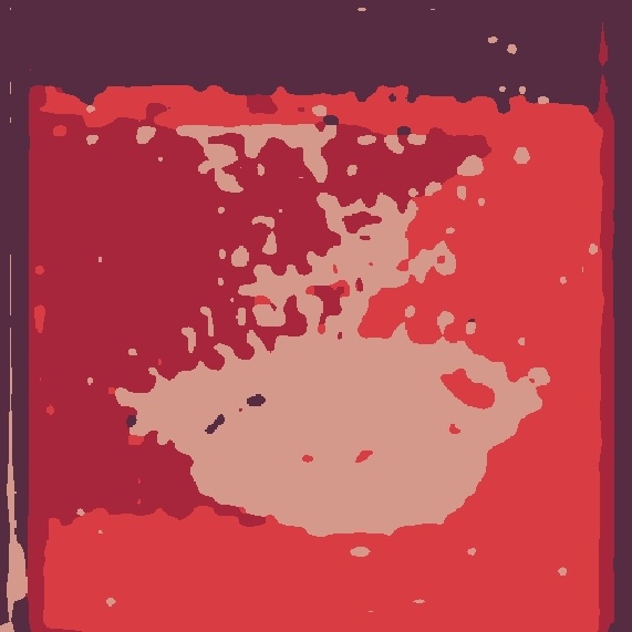
Figure 5: Some sample images. a) Peppers. b) House. c) Splash. a,b,c) Courtesy of USC-SIPI, Signal and Image Processing Institute at the University of Southern California. d) Food Peppers, courtesy of freeimages.co.uk. e) Toy, courtesy of Computational Vision at Caltech, http://www.vision.caltech.edu. f) Dessert.

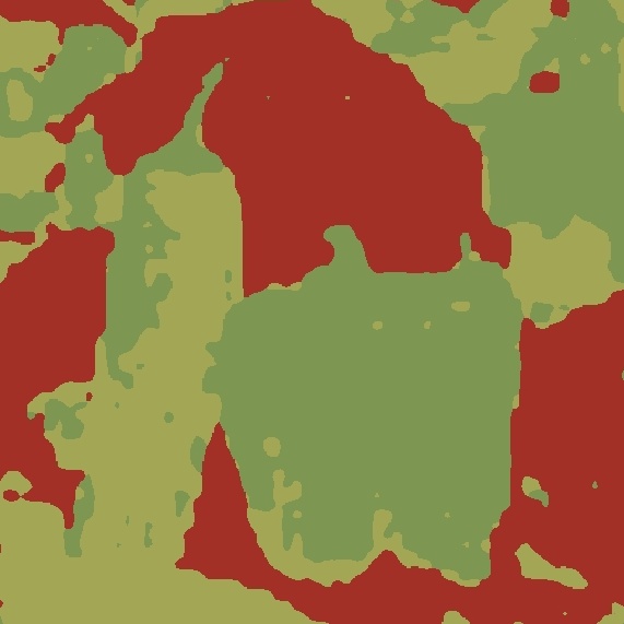
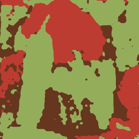
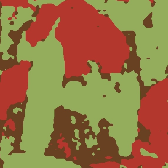
Figure 6 shows the results of three independent runs of the proposed method on the image Peppers. Here, m=2, c=2, n₁=4, and n₂=3 are used. This figure shows that while the proposed method always results acceptably, its output is never identical in different runs, even with the identical values of the parameters, similar to the entire category of fuzzy clustering algorithms [21]. It should be emphasized, though, that in contrast with the conventional pixel-based fuzzy clustering approaches, in which local minimum is a common unsolved problem [21], the proposed method shows less tendency to falling into local minima. A local minimum in a fuzzy clustering algorithm can be identified by a solution which does not satisfy the merits which the problem defines but still cannot be improved by the local approach utilized in the general clustering algorithm [21]. We argue that the relative immunity of the proposed method against getting trapped in local minimums is the result of two innovations in it. First, rather than working on the original realizations, which are noisy and may contain many outliers, the proposed method works on more robust statistical parameters of blocks of the image. Secondly, the proposed distance function models the physical phenomenon more appropriately, compared to the pixel-level operators used before. It is worth to emphasize that the proposed method is more repeatable, compared to the FPCAC [7], which uses a similar distance measure in the pixels level. In the experiments shown in Figure 6, the algorithm has converged in 9, 6, and 5 iterations, elapsing 16s, 14s, and 14s, respectively.



(a)	(b)	(c)

Figure 6: Results of three independent runs of the proposed method on the image Peppers. Top) Results of segmentation. Bottom) Principal colors.

Figure 7 shows the results of the proposed method applied on the image House, while different values of m are used. Here, with c=3 and m Î {1¹/₃, 1²/₃, 2}, the algorithm has converged in 4, 10, and 9 iterations, elapsing 13s, 16s, and 16s, respectively. More experiments show that the actual value of m has minimal effect on the results of the proposed method. Hence, the value of m=2 is used as the default value. Similarly, the values of n₁ and n₂ only affect the spatial precision of the results and the elapsed time. As a compromise, we always select n₁=4 and n₂=3.



(a)	(b)	(c)

Figure 7: Effects of m on the results of the proposed method on the image House. Top) Results of segmentation. Bottom) Principal colors.

In a proper segmentation process, it is expected that increasing c should result in an increasingly better depiction of different regions in the image. Using values of c=2, c=3, and c=4, this aspect of the proposed method is investigated in Figure 8. As expected, increasing the number of clusters results in more detailed segmentation results. In these experiments, the algorithm has converged in 9, 5, and 8 iterations, elapsing 12s, 14s, and 18s, respectively. It should be emphasized that the elapsed time of the proposed algorithm depends almost linearly on the number of clusters.



(a)	(b)	(c)

Figure 8: Effects of c on the results of the proposed method on the image Splash. Top) Results of segmentation. Bottom) Principal colors.

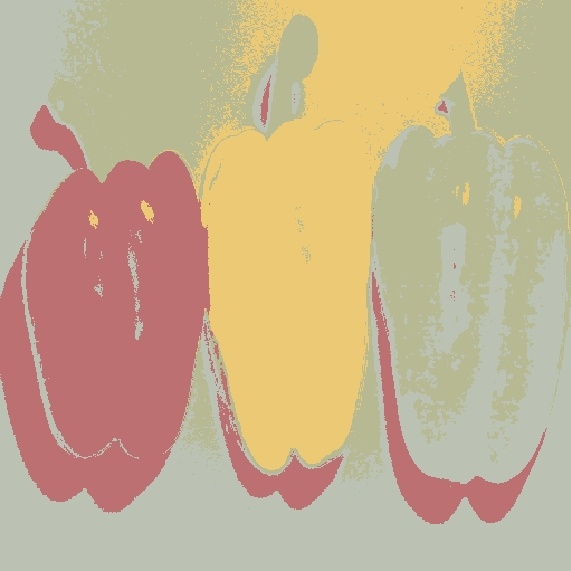
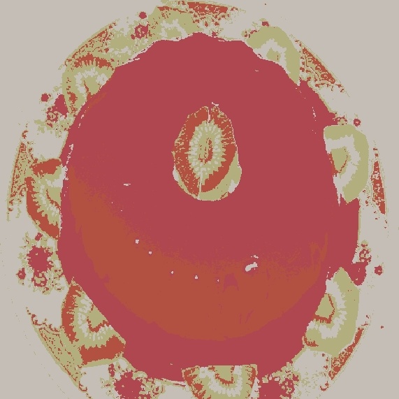
Figure 9 compares the performance of the proposed method with the FPCAC [7]. This comparison is important because both methods search for cylindrical structures in the color space. Note that while the FPCAC works on individual pixels, the proposed method utilizes more robust statistically computed features. In this experiment, the FPCAC is utilized with its own default value of m=1.05 [7]. Table I lists the elapsed time and the number of iterations of each method when working on each image. Also, the value of c=4 is used for both methods in all cases.

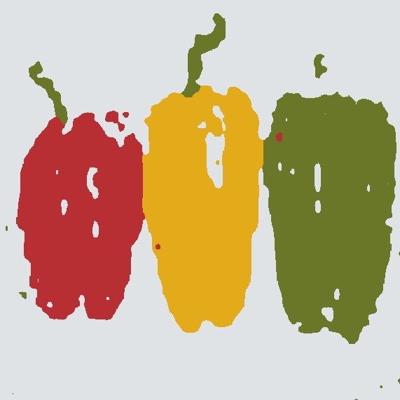
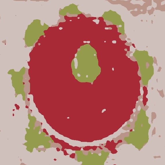
As mentioned in Section I, there is no standard method for comparing the performance of different segmentation methods. Thus, here, we compare the results of the proposed method and the FPCAC, as shown in Figure 9, based on a heuristic approach. Comparing Figure 9-a with Figure 9-d, a very common problem of many segmentation methods can be seen. This way, in Figure 9-a, FPCAC has mistakenly included parts of the gray background in the yellow pepper. Also, the shadow of the red pepper and other parts of the background are included in the red and green peppers, respectively. However, looking at Figure 9-d, we see a proper segmentation of the image into four distinguished parts of red, yellow, and green peppers, and the background by the proposed method. Figures 9-b and e show an example where the two methods perform similarly, except for the fact that FPCAC has resulted in an over-segmentation. This way, as seen in Figures 9-b, FPCAC has segmented the text on the object into two different classes (because of being pixel-based). The proposed method, on the other hand, has given a smoother segmentation result. This effect is also visible in Figure 9-c, where FPCAC has again resulted in many tiny segments. In contrary, the proposed method has again produced a smooth segmentation result. It is worth to mention that the proposed method is also faster than the FPCAC. The reader is referred to [6] for more examples.

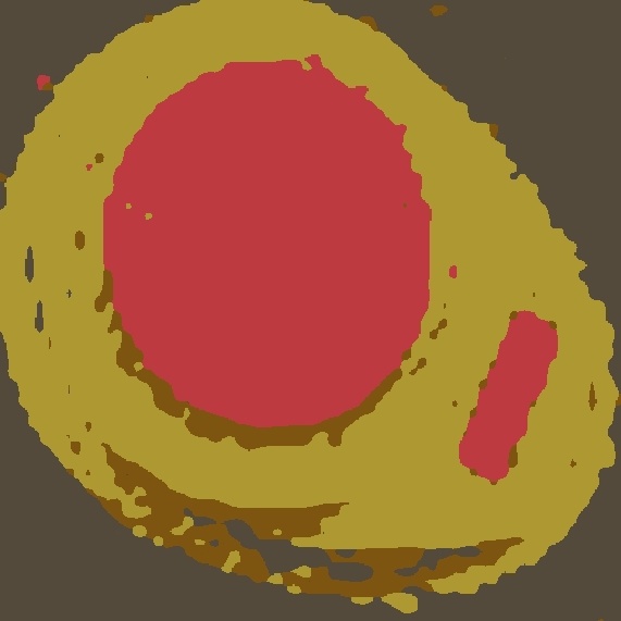
In analyzing the performance of the proposed method, it is worth to mention that as the proposed algorithm is primarily concerned with spectral accuracy, details in the spatial domain might be ignored. For example, looking at Figure 9-e, we observe that the proposed method has missed the details in the text on the object. This is a direct result of looking at the image in lower resolutions, as done using n₁ and n₂. While this is useful in applications which look for the general geometry of the objects, in other applications which demand more precision, including coding, a pixel-based approach would yield more applicable results. Thus, we argue that the proposed method produces acceptable results when the aim is to find homogeneous regions in an image with more emphasis on the color information, and not on the spatial details.


(a)	(b)	(c)


(d)	(e)	(f)

Figure 9: Comparison of the proposed method with the FPCAC [7]. (a), (b), and (c) Results of the FPCAC. (d), (e), and (f) Results of the proposed method.

Table 1: Performance comparison of the proposed method and the FPCAC [7]. [t: Elapsed time. i: Number of iterations before convergence.]

Image	Proposed Method		FPCAC [7]
	t(s)	i	t(s)	i

Figure 5-d	20	10	26	40
Figure 5-e	18	6	8	19
Figure 5-f	21	11	24	38

4 Conclusions

In this paper, a new color image segmentation method is proposed which utilizes the general clustering algorithm with an innovative distance function. The mathematics of the proposed method is discussed comprehensively and experimental results are presented. Comparison of the performance of the proposed method with an available clustering method, which searches for similar cylindrical structures in the pixel domain, shows that the proposed method is more stable and faster. We argue that this is mainly because of applying the clustering task on a more robust statistical feature. It is also observed that the proposed method decreases the probability of local minimum entrapment. The repeatability of the proposed segmentation method is also more than the available one. Furthermore, while the proposed method gives a more perceptually satisfactory segmentation, it demands less processing resources.

Acknowledgement

This work was in part supported by a grant from ITRC. Also, Arash Abadpour wishes to thank Ms. Azadeh Yadollahi for her encouragement and invaluable discussions. We also appreciate the respected anonymous referees for their constructive suggestions.

References

[1]: G. J. Klinker, S. A. Shafer, and T. Kanade, "The measurement of highlights in color images," International Journal of Computer Vision, vol. 2, pp. 7-32, 1988.
[2]: --, "A physical approach to color image understanding," International Journal of Computer Vision, vol. 4, pp. 7-38, 1990.
[3]: S.-C. Cheng and S.-C. Hsia, "Fast algorithms for color image processing by principal component analysis," Journal of Visual Communication and Image Representation, vol. 14, pp. 184-203, 2003.
[4]: D. O. Nikolaev and P. O. Nikolayev, "Linear color segmentation and its implementation," Computer Vision and Image Understanding, vol. 94, pp. 115-139, 2004.
[5]: M. Turk and A. Pentland, "Eigenfaces for recognition," Journal of Cognitive Neuroscience, vol. 3(1), pp. 71-86, 1991.
[6]: A. Abadpour, "Color image processing using principal component analysis," Master's thesis, Sharif University of Technology, Mathematical Sciences Department, Tehran, Iran, June 2005.
[7]: A. Abadpour and S. Kasaei, "A new FPCA-based fast segmentation method for color images," in The 4th IEEE International Symposium on Signal Processing and Information Technology (ISSPIT 2004), Rome, Italy, 2004.
[8]: --, "Unsupervised, fast and efficient color image copy protection," IEE Proceedings Communications, vol. 152 (5), pp. 605-616, 2005.
[9]: --, "An efficient PCA-based color transfer," Visual Communication & Image Representation, vol. 18 (1), pp. 15-34, 2007.
[10]: L. Lucchese and S. Mitra, "Color image segmentation: A state-of-the-art survey (invited paper)," Image Processing, Vision, and Pattern Recognition, Proc. of the Indian National Science Academy (INSA-A), vol. 67, A, No. 2, pp. pp. 207-221, 2001.
[11]: W. Skarbek and A. Koschan, "Colour image segmentation-a survey," Institute for Technical Informatics, Technical University of Berlin, Tech. Rep., 1994.
[12]: T. Q. Chen and Y. Lu, "Color image segmentation - an innovative approach," Pattern Recognition, vol. 35, pp. 395-405, 2002.
[13]: A. Hyvarinen, J. Karhunen, and E. Oja, Independent Component Analysis. John Wiley & Sons, Inc., 2001.
[14]: P. E. Gill, W. Murray, and M. H. Wright, Numerical Linear Algebra and Optimization. Redwood City, California: Addison-Wesley Publishing Company, 1991.
[15]: J. C. Bezdek, Pattern Recognition with Fuzzy Objective Function Algorithms. New York: Plenum Press, 1981.
[16]: K. Honda, N. Sugiura, and H. Ichihashi, "Robust local principal component analyzer with fuzzy clustering," in IJCNN 2003 Conference Proceedings, 2003, pp. 732-737.
[17]: I. Gath and A. Geva, "Unsupervised optimal fuzzy clustering," IEEE Transaction on Pattern Analysis Machine Intelligence, vol. 11(7), pp. 773-781, 1989.
[18]: J. M. Leski, "Fuzzy c-varieties/elliptotypes clustering in reproducing kernel hilbert space," Fuzzy Sets and Systems, vol. 141, pp. 259-280, 2004.
[19]: D. E. Gustafson and W. C. Kessel, "Fuzzy clustering with a fuzzy covariance matrix," in Proceedings of the IEEE CDC, vol. 2, San Diego, CA, 1979, pp. 761-766.
[20]: J. M. Leski, "Generalized weighted conditional fuzzy clustering," IEEE Transactions on Fuzzy Systems, vol. 11 (6), pp. 709-715, 2003.
[21]: J. Bezdek, J. Keller, R. Krisnapuram, and N. R. Pal, Fuzzy Models and Algorithms for Pattern Recognition and Image Processing. Boston: Kluwer Academic Publishers, 1999.

File translated from T_EX by T_TH, version 3.72.
On 27 Feb 2008, 14:35.

Principal Color and Its Application to Color Image Segmentation

Arash Abadpour 1 and Shohreh Kasaei 2 1 Mathematics Science Department, Sharif Univ. of Tech., Tehran, Iran, email: abadpour@math.sharif.edu2 Computer Engineering Department, Sharif Univ. of Tech., Tehran, Iran, email: skasaei@sharif.edu

Abstract

1 Introduction

2 Method

2.1 Finding the Closest Point to a Set of Lines

2.2 Finding the Closest Point to a Set of Fuzzy Lines

2.3 General Clustering Algorithm

2.4 Color Image Segmentation using Principal Colors

3 Experimental Results

4 Conclusions

Acknowledgement

References

Arash Abadpour ¹ and Shohreh Kasaei ²
¹ Mathematics Science Department, Sharif Univ. of Tech., Tehran, Iran, email: abadpour@math.sharif.edu
² Computer Engineering Department, Sharif Univ. of Tech., Tehran, Iran, email: skasaei@sharif.edu